| SST= |
(1) |
(JPL Publication D-14070)
NOAA/NASA AVHRR Oceans Pathfinder
Sea Surface Temperature Data Set
User's Reference Manual
Version 4.0
April 10, 1998
Jorge Vazquez (JPL/Caltech)
Kelly Perry (JPL/Caltech)
Kay Kilpatrick (RSMAS/University of Miami)
Appendices were provided by:
Katherine Kidwell (NOAA), Robert Evans (University
of Miami),
Guillermo Podesta (Univerisity of Miami), Kay Kilpatrick (University of
Miami)
1.0 INTRODUCTION
2.0 ALGORITHMS AND DATA PROCESSING
- 2.1 Algorithm Overview
- 2.2 Accuracy of AVHRR-derived SSTs
- 2.3 Processing Flow
3.0 DATA SET DETAILS (Equal-Angle
Products)
- 3.1 Overview
- 3.2 Equal Angle Best SST Data
- 3.4 Equal Angle All SST
- 3.5 Matchup Database
- 3.6 Equal Area
4.0 DATA INFORMATION AND ACCESS
- 4.1 Regional Subsetting and Extraction Using WWW
- 4.2 Downloading the Data Using Anonymous FTP
- 4.3 Information About Processing Status
5.0 READING AND USING DATA SETS
- 5.1 Conversion of DN to SSTs and Pixel Coordiante
to Latitude and Longitude
- 5.2 Read Software
- 5.3 Attributes
6.0 REFERENCES
7.0 ACKNOWLEDGMENTS
APPENDIX A- Satellite and Instrument
APPENDIX B - Coefficients and Validation
APPENDIX C - Quality Flags Assignments and
Information
APPENDIX D - Read Software
APPENDIX E - Science Working Group and JPL Team
APPENDIX F - Acronyms
APPENDIX G - AVHRR Pathfinder Oceans SST Algorithm
2.0 ALGORITHMS AND DATA PROCESSING
Current retrieval algorithms for sea surface temperature from AVHRR are based largely upon the multi-channel sea surface temperature (MCSST) algorithm (McClain et al., 1985) which may be written as:
| SST= |
(1) |
where ![]() 1 and
1 and
![]() 2 are constants
determined through a least-squares fit to in-situ data, T4,
T5, are brightness temperatures as derived
from channels 4 and 5 (see table 1) and
2 are constants
determined through a least-squares fit to in-situ data, T4,
T5, are brightness temperatures as derived
from channels 4 and 5 (see table 1) and ![]() is a weighting factor based on the knowledge of known absorption coefficients
(Emery et al., 1994). In this form the linear model has no correction for
water vapor attenuation. A nonlinear SST algorithm (NLSST) was introduced
that incorporates an initial estimate of the SST field, where the coefficients
are calculated for different water vapor regimes as defined by (T4
- T5) differences. The form of the NLSST algorithm used
to derive the Pathfinder SST becomes:
is a weighting factor based on the knowledge of known absorption coefficients
(Emery et al., 1994). In this form the linear model has no correction for
water vapor attenuation. A nonlinear SST algorithm (NLSST) was introduced
that incorporates an initial estimate of the SST field, where the coefficients
are calculated for different water vapor regimes as defined by (T4
- T5) differences. The form of the NLSST algorithm used
to derive the Pathfinder SST becomes:
| SST= |
(2) |
where the "![]() s"
are still coefficients based on a least squares fit to in-situ data and
T4, T5 are the brightness temperatures in channels
4 and 5. Theta is the satellite scan angle or the incidence angle of the
incoming radiation based on the horizontal plane of the satellite, and
Tsurf is a first guess sea surface temperature field; in this
case the Reynolds optimally interpolated (OI) sea surface temperature data.
A non-linearity in the algorithm arises because of the Tsurf term and the
4 coefficients being calculated over two different (T4 - T5)
differences. In version 4.0 and 4.1 of the algorithm the coefficients are
calculated for T4 - T5 <= 0.7
and T4 - T5 > 0.7. This
form of the algorithm was approved for the reprocessing of the MCSST data
by the AVHRR Oceans Science Working group because it tended to lower the
overall bias over the widest possible environmental conditions (Evans and
Podesta., 1996). A nonlinearity arises from the coefficients being calculated
over different water vapor regimes corresponding to (T4 - T5);
the V1 algorithm calibration coefficients were calculated yearly for three
different water vapor regimes or T4-T5 channel differences.
s"
are still coefficients based on a least squares fit to in-situ data and
T4, T5 are the brightness temperatures in channels
4 and 5. Theta is the satellite scan angle or the incidence angle of the
incoming radiation based on the horizontal plane of the satellite, and
Tsurf is a first guess sea surface temperature field; in this
case the Reynolds optimally interpolated (OI) sea surface temperature data.
A non-linearity in the algorithm arises because of the Tsurf term and the
4 coefficients being calculated over two different (T4 - T5)
differences. In version 4.0 and 4.1 of the algorithm the coefficients are
calculated for T4 - T5 <= 0.7
and T4 - T5 > 0.7. This
form of the algorithm was approved for the reprocessing of the MCSST data
by the AVHRR Oceans Science Working group because it tended to lower the
overall bias over the widest possible environmental conditions (Evans and
Podesta., 1996). A nonlinearity arises from the coefficients being calculated
over different water vapor regimes corresponding to (T4 - T5);
the V1 algorithm calibration coefficients were calculated yearly for three
different water vapor regimes or T4-T5 channel differences.
All the algorithms used the non-linear SST algorithm (NLSST), developed and used operationally by NOAA/NESDIS. Earlier forms of the algorithm such as Version 3.0 also use the nonlinear SST algorithm (equation 2) with calibration coefficients calculated for two different water vapor regimes or T4-T5 channel radiance differences and over 5 month periods centered on each month. The improvement of the version 4.1 data set over previous algorithms such as version 1.0, 3.0 and 4.0 lies in the use of a tree algorithm to calculate the quality flags, thus making the procedure of quality flag assignment more objective. The tree algorithm leads to a quality flag between 0-7 being assigned to a plxel value, with 0 being the lowest quality and 7 being the highest quality. For version 4.1 pixels are defined as best that are assigned a quality flag greater than or equal to 3. In earlier versions pixels were flagged as best which were assigned a quality flag of 3. For more details see http://www.rsmas.miami.edu/~gui/algov4/algoV4doc.html (Evans and Podesta, 1998) or appendix G. Appendix C contains details on the tests used to assign the quality flags for version 4.1. The information is provided by Guillermo Podesta and Katherine Kilpatrick at the University of Miami.
The currently available Version 4.0 Pathfinder data sets cover 1985 to 1995. Version 4.1 data has been processed for 1996. For updates on the status of reprocessing the earlier years with the 4.1 algorithm please see the PODAAC AVHRR Pathfinder homepage http://podaac.jpl.nasa.gov/sst/. Reprocessing of all the 1985-1995 using the Version 4.1 software is planned for the near future.
2.2 Accuracy of AVHRR-derived SSTs
Work is currently underway to determine the accuracy of the data (see Vazquez et al., 1998 or Evans et al., 1996). Current results indicate that the accuracy is regionally dependent and influenced by the water vapor content in the atmosphere. However more work needs to be done to confirm this. Some points of interest from work with previously available AVHRR derived SSTs include:
| 1) | The SST measurement is of the skin temperature, and not the bulk temperature (Schuluesso et al., 1990). |
| 2) | Atmospheric water vapor partly affects the retrieval, but no independent water vapor data sets are used in the algorithm (Emery et al, 1994). |
| 3) | Most successful uses of past MCSST data concentrated on identifying spatial temperature gradients (Gulf Stream fronts, etc.) rather than absolute temperature values. The present calibrations are designed to provide consistency over the duration of the 5-channel data record. |
| 4) | Cloud masking in any `all-pixel' image can be minimized by taking the warmest pixel at a fixed location over all images within one week. The logic is that clouds are "cold", and they move much farther in one week than ocean features. |
Your experience with this data is valuable to the NOAA/NASA AVHRR Oceans
Pathfinder Project. If you have any questions or comments please contact
Jorge Vazquez at podaac@podaac.jpl.nasa.gov
as to your experiences using the Oceans Pathfinder data.
| Example of Monthly Composite of Sea Surface Temperature from NOAA/NASA AVHRR Oceans Pathfinder SST Data Set |
 |
The Global Area Coverage (GAC) data are obtained by the algorithm and processing team at the University of Miami. The calibrated data contain the radiances for the 5 channel AVHRR instrument (see table 1). For more details on the instrument design and orbit details see Appendix A.
AVHRR Spectral Bands in microns
| Channel Position (µm) | |||||
| Platform | 1 | 2 | 3 | 4 | 5 |
| NOAA-7,9,11,12,14 | 0.55-0.68 | 0.725-1.10 | 3.55-3.93 | 10.3-11.3 | 11.5-12.5 |
The data are binned from the Global Area Coverage 4km AVHRR resolution
to approximately 9km. For more details on the algorithm for version 4.1
see http://www.rsmas.miami.edu/~gui/algov4/algoV4doc.html
(Evans and Podesta, 1998). A copy of this document is also included in
Appendix G.
The University of Miami provides the processing coefficients based on an analysis of buoy data and a least-squares fit to equation (2). For the version 4.0 and 4.1 data these coefficients are calculated over a 5 month period centered on each month. The University of Miami provides the Pathfinder Team at JPL with processing software to convert the equal-area SST data into the equal-angle products that are distributed through the PODAAC.
3.0 DATA SET DETAILS (Equal-Angle Products)
The NOAA/NASA AVHRR Oceans Pathfinder SST data are distributed in several spatial and temporal resolutions. Each data product is produced as both ascending (daytime) and descending (nighttime) images. These products are distributed as daily and monthly files, which are defined as spatially and temporally averaged bins of all temperature retrievals. There are four main products: 1) best_sst 2) all-pixel sst 3) equal-area and 4) the matchup database. The products are available at different spatial resolutions including at 9km, 18km and 54km spatial resolutions. In addition, in the near future, the equal-angle products will also be available as weekly and monthly averaged SST data. Plans are also underway to create an 8-day average that is compatible with the SEAWIFS ocean color data. Details for these products are described in sections 3.2-3.6. The naming cnvention is such that:
yyyydddfrrpp-zzz.hdf
where
yyyy is the 4 digit year
ddd is the Julian Day for that year
f is the format h=hdf
rr is the spatial resolution (9, 18, or 54
kilometers)
pp is the pass (da for ascending and
dd for descending)
zzz is a three letter code (gdm for
best-sst and adm for all-pixel).
In the equal-angle projection there is an equal number of pixels in both the longitude and latitude directions. As an example the 9km data sets consist of data with 4096 pixels in the East-West direction (longitudinal) and 2048 pixels in the North-South direction (latitudinal) Consequently a better description of the spatial resolution is in terms of pixels/degree of latitude and longitude. For the 9km equal-angle data set, the spatial resolution in pixels/degree of latitude and longitude is 4096/360 or 11.37777. At the equator, where the number of kilometers per degree of latitude and longitude is 111.19 km, this translates to 9.77 km per pixel. Toward the poles the kilometers per pixel are vastly reduced to the point where they do not contain multiple SST retrievals. The product is available in spatial resolutions of approximately 9km, 18km, 54km and temporal resolutions of daily and monthly images. The grid size for the 9km resolution is 4096x2048, the 18km is 2048x1024, and the 54km is 720x360. Thus the resolution in pixels/degrees is 4096/360 (11.38) for the 9km grid size, 2048/360 (5.69) for the 18km grid size, and 2.0 for the 54km grid size. The data is in DN or digital numbers and for conversion to SST needs to be mutiplied by a slope of 0.15 with a y-intercept of -3.0 added. Thus the conversion equation is simply:
SST=0.15 * DN - 3.0
This product, after a series of statistical tests, retains only the highest quality pixels. For a definition of these statistical tests in Version 4.1 of the algorithm see Appendix C. . Briefly in version 4.1 quality flags are assigned between 0-7 depending on what series of tests are passed. Because only pixels of quality 3 or better are kept, there is less data than the `all pixel' product discussed in section 3.4. In the best SST product, cloud-associated areas are rejected, as is the far portion of the swath. Values with pixel quality of 2 or less in hte Version 4.1 data are set to 0. Thus for the best-sst equal-angle product auxiliary information includes the number of points that went into the calculation of the SST for that pixel.
As data are produced it is announced on the PODAAC AVHRR SST Pathfinder
homepage at http://podaac.jpl.nasa.gov/sst.
Product update bulletins are sent to an e-mail distribution list; you can
add yourself to this list through the PODAAC homepage http://podaac.jpl.nasa.gov.
The data are available via ftp and through the subsetting routine on http://podaac.jpl.nasa.gov/sst
The product is available in the HDF format as raster images (DFR8API).
It contains two bands or image planes of data, the first is the pixel or
DN value to be converted to SST and the second is the number of points
per bin. This data may be accessed through the FTP site at podaac.jpl.nasa.gov
in the /pub/sea_surface_temperature/avhrr/pathfinder/ directory. These
data may also be subsetted through the www at http://podaac.jpl.nasa.gov/sst/.
An example of the homepage subsetting tool is seen in section 4.1. Example
read software may be found under:
/pub/ sea_surface_temperature/avhrr/pathfinder/software.
Equal Angle Best SST data
| Data Set: | Equal Angle Best Sea Surface Temperature |
| JPL Product Numbers: | 091-Version 4.0 data 095-Version 4.1 data |
| Image Size: | 4026 x 2048 (daily for 9km data) 2048 x 1024 (daily for 18km data) 720 x 360 (daily for 54km) |
| Data Size: | ~16.5 MBytes (~1.2 MBytes compressed) for 9km
data ~4.2 MBytes (~406 KBytes compressed) for 18km data ~518 KBytes |
| Temporal averaging: | Daily, monthly |
| Format: | HDF |
| # Extractable Parameters: | 2 Bands |
| HDF Band 1: | Sea Surface Temperature: Value of retrieval |
| HDF Band 2: | Number of Observations Per Bin: Number of SST values that were averaged from the 9km, 18km, or 54km bin. |
| Data Access: | Via anonymous ftp: ftp podaac.jpl.nasa.gov/pub Via subsetting: http://podaac.jpl.nasa.gov/sst On tape, contact podaac@podaac.jpl.nasa.gov |
| File names: | 1995363h09da_gdm.hdf (example) 1995363h18da_gdm.hdf (example) 1995363h54da_gdm.hdf (example) |
The naming convention is such that the SST data contained in 1995363h09da_gdm.hdf is for an ascending pass on day 363 of 1995 at a 9km spatial resolution. The data on the same day for a descending pass would be contained in:
1995363h09dd_gdm.hdf
This product contains all pixels regardless of data quality flag so there is no cloud masking. Thus for the Equal-Angle All Pixel SST product the auxiliary information includes information on both the number of observations that went into the average for that bin and the quality flag assigned to that pixel or bin. HDF files contain three bands or image planes of data including the DN value, quality flag assigned to that DN value, and the # of observations that went into that bin. Quality flags are assigned between 0-7 (see Appendix C) based on a series of statistical tests. As before DN values maybe converted to SST by applying a slope and y-intercept such that SST=0.15*DN-3.0. As is the case with the Best SST product, the product is available in spatial resolutions of approximately 9km, 18km, 54km and temporal resolutions of daily and monthly images. The grid size for the 9km resolution is 4096x2048, the 18km is 2048x1024, and the 54km is 720x360. Thus the resolution in pixels/degrees is 4096/360 (11.38) for the 9km grid size, 2048/360 (5.69) for the 18km grid size, and 720./360. 2.0 for the 54km grid size.
Because of the size of the 9km files, this data is only available on tape. The data maybe ordered through podaac@podaac.jpl.nasa.gov, or the www homepage http://podaac.jpl.nasa.gov. The 18km and 54km are available through the ftp site at podaac.jpl.nasa.gov. Example read software may be found under
/pub/ sea_surface_temperature/avhrr/pathfinder/software
Equal Angle All SST
| Data Set: | Equal Angle All Sea Surface Temperature |
| JPL Product Number: | 090 - Version 4.0 data 094 - Version 4.1 data |
| Image Size: | 4026 x 2048 (for nominal 9km data) 2048 x 1024 (for nominal 18km data) 720 x 360 (for nominal 54km data) |
| Data Size: | ~24.7 MB (~5.3 MB compressed), nominal 9km data ~6.3 MB (~1.8MB compressed) for nominal 18km data |
| Temporal averaging: | Daily, monthly |
| Format: | HDF |
| # Extractable Parameters: | 3 Bands |
| HDF Band 1: |
Sea Surface Temperature: Value of retrieval |
| HDF Band 2: | Pixel Quality: Flag Value between 0 and 7 as defined in Appendix C. |
| HDF Band 3: | Number of Observations Per Bin: Number of SST values that were averaged from the nominal 9km bin. |
| Data Access: | Daily and monthly averaged data via anonymous
ftp: ftp podaac.jpl.nasa.gov/pub, daily data is only available on tape. For tapes, contact podaac@podaac.jpl.nasa.gov |
| File names: | 1995363h09da_adm.hdf (example) 1995363h18da_adm.hdf (example) 1995363h54da_adm.hdf (example) |
A large validation data set called the Pathfinder Matchup Data Base (PFMDB) is also available (Podesta et al., 1997). These are the buoy data used in determining the coefficients. The data set is a compilation of a multi-year, multi-satellite database of approximately co-temporal, co-located in situ sea surface temperatures and AVHRR measurements. AVHRR data were extracted at the times and locations of the in situ observations. The maximum temporal separation between the satellite retrieval and the in situ observation was required to be 30 minutes for the pair to be considered a "match". Spatially, the satellite retrieval and in situ observation were required to be within approximately 10km of each other to be considered a match. The result of this matching process is a series of records which contain both satellite-derived and in situ observations.
Each Pathfinder SST algorithm version number is associated with a specific set of matchups. For example version 4.0 and 4.1 data is associated with the Version 19.0 matchups. Version 3.0 data is associated with Version 18.0 of the matchups and Version 17.0 is associated with Version 1.0 of the algorithm. Each record in the Version 19.0 data set contains 195 fields which include the value of the satellite measured SST at the buoy location and the SST from the matchup buoy.
The PFMDB version 19.0 is organized into several files, by month of the year. The naming convention is such that : g_noa14_v19.0_9603.matchups.jpl contains data from NOAA-14 for March of 1996. It includes quality-controlled in situ SST data from both moored and drifting buoys. The quantities in the matchup database are listed in http://www.rsmas.miami.edu/~gui/v19/matchups.v19.0.html. A hardcopy of this document may also be obtained by contacting podaac@podaac.jpl.nasa.gov.
Version 19.0 of the matchups is available as JPL product 089 from the anonymous FTPs site at podaac.jpl.nasa.gov in
/pub/sea_surface_temperature/pathfinder/matchups/v19.0_matchups/data/
Software to read the data maybe found in the:
/pub/sea_surface_temperature/pathfinder/matchups/v19.0_matchups/software/
The following table shows the sources of in situ SST data included in the PFMDB:
Source of In Situ SST in PFMDB
| BUOY TYPE: | SOURCE: |
Moored Buoys |
- U.S. National Data Buoy Center (via NODC) - Japan Meteorological Agency - TOGA/TAO Project NOAA Pacific Marine Environment Laboratory |
Drifting Buoys |
-NOAA Atlantic Oceanographic and Meteorological Laboratory Canadian Marine Environmental Data Service |
| FTP NAMES | /data/g_noa9_v19.0_9503.matchups.jpl (example) |
Most of the initial in situ data compilation and quality control was done
in collaboration with Dr. Charles McClain and his research group at NASA's
Goddard Space Flight Center.
This product is only available via special request. People interested in this product should contact the JPL PO.DAAC via e-mail (podaac@podaac.jpl.nasa.gov). The equal area product is based on a gridding scheme where the number of bins per longitude is dependent on the latitude. The data set generated for distribution is a nominal 9km equal-area product with 6 different bands or extractable parameters describing the sea surface temperature in a given bin. These are distributed as HDF files, and are approximately 120 MB in size. The equal-area files are also available, upon special request, to users who are familiar with the DSP language. The sum squared SSTs and number of observations per bin are included for proper resampling, should a researcher have special spatial or temporal requirements. Pixel quality and mask bits are determined during processing, and based on a variety of tests. The 6 bands included in an equal-area product are listed in the following table.
Extractable Parameters for an Equal Area Product
| BAND | PARAMETER | DESCRIPTION |
1 |
Bin Number |
A unique number assigned to a particular bin based on the equal-area grid. This bin_number then is associated with a specific geographical or latitude, longitude coordinate. |
2 |
# of Observations/Bin |
Because the 9 km bins are based on an average of 4 km Level-1B data, this parameter indicates the number of observations that went into the average of each bin. |
3 |
Pixel Quality |
A quality flag generated during processing, which indicates the quality of the temperature estimate at each pixel. Values can be between 0 and 7 (Version 4.1) inclusive, depending on a series of statistical tests and comparisons with other sources of data (see Appendix C). |
4 |
Mask Bits |
This band contains different image masks that are used, such as cloud or ice masks. |
5 |
Sum SST |
For a given 9 km bin this number is the sum of the sea surface temperature values in that bin. This number, along with the number of observations per bin, can then be used to derive the average sst value. |
6 |
Sum Squared SST |
For a given 9 km bin this number is the sum of the squared sst values, to be used in computing higher-order statistical moments. |
4.0
DATA INFORMATION AND ACCESS
Data may be acquired electronically or on tape, as listed in the tables in section 3. Most data are available via anonymous FTP with the exception of 9km all-pixel data which are available on tape. Tape orders may be placed through http://podaac.jpl.nasa.gov or via email to podaac@podaac.jpl.nasa.gov. All data are available on 8mm UNIX tar tapes as mentioned in section 3.0. Information on the products and their availability is found on the www http://podaac.jpl.nasa.gov/sst/ under AVHRR NEWSThe best_sst at all resolutions and the 18km, and 54km all_plxel data are available via FTP. Data may also be ordered through the EOSDIS Version 0 Information Management System (IMS). It is accessed via http://harp.gsfc.nasa.gov/ims-bin/pub/imswelcome.
4.1 Regional Subsetting and Extraction Using WWW
JPL has developed an on-line regional subsetting capability which is
accessible through the NOAA/NASA AVHRR Oceans Pathfinder homepage (http://podaac.jpl.nasa.gov/sst).
This capability allows the user to extract regional data from the global
data set. The user selects a region using geographic coordinates, the time
period and data format HDF, RAW, GIF). The input spawns an automatic subsetting
routine at JPL which subsets and stages the data to the ftp site. An e-mail
message to the requester provides the location of the extracted data sets.
The following figure shows the subsetting page from the Pathfinder homepage.
The extraction involves entering the maximum and minimum coordinates in
latitude and longitude.
4.2 Downloading the Data Using
Anonymous FTP
For data that is available via ftp, connect to podaac.jpl.nasa.gov
using ftp, and enter 'anonymous' for a user name. Please use your full
e-mail address for a password. At the ftp prompt enter:cd / pub/sea_surface_temperature/avhrr/pathfinder/
There are 11 sub directories. They are browse_v1/, browse_v3, browse_v4,
browse_v4.1, data_v1, data_v3, data_v4, data_v4.1, matchups/, software/,
and /doc.
| document: | this directory contains documentation such as the users guide in post script and a readme file. |
| matchups: | this directory contains the matchup database, see section 3.6. |
| software: | this directory contains FORTRAN AND IDL routines for reading the HDF data files.. Use of the IDL routines and package requires that you have IDL version 3.5 or better installed on your system, and use of the FORTRAN and C routines requires that you acquire, compile, and install the HDF library (available via anonymous ftp from ftp.ncsa.uiuc.edu). For more information about HDF or to acquire the HDF library, contact the National Center for Supercomputing Applications (NCSA) at http://hdf.ncsa.uiuc.edu. |
| data_v1.0....4.1: | directories contain the ascending and descending data for the particular version number. Subdirectories are separated by temporal resolution (daily, monthly), spatial resolution (9km, 18km, 54km), satellite pass (ascending, descending), and data type best_sst, and all_pixel. |
| browse_v1.0...4.1: | contains gif browse images of the data |
| colorbar.gif: | a gif file containing the colorbar |
Please note that previous versions of the data will be taken offline once version 4.1 time series is complete for a given year.
4.3 Information about processing status
Status bulletins are e-mailed to a list of users. To add yourself to this list please refer to the JPL PO.DAAC homepage; http://podaac.jpl.nasa.gov. Status updates are also provided in the `Whats new' section of the JPL PO.DAAC homepage and on the Pathfinder homepage http://podaac.jpl.nasa.gov/sst.
5.0 READING AND USING DATA SETS
5.1 Conversion of DN to SSTs and pixel coordinate to latitude and longitude
The files are daily images of sea surface temperature data. The HDF data are in the form of raster images, therefore the data are contained in byte arrays. Values range from 0 to a possible maximum of 255. Values of 0 refer to missing data or cloud cover. The format of the file consists of a byte array of dimension 4096 x 2048 for a nominal 9 km spatial resolution data set. The byte or DN values can then be scaled into the appropriate sea surface temperature by using the following y-intercept and slope values.
SST=0.15*DN-3.0
where SST is in degrees Celsius. For the nominal 18 km data the dimension of the byte array is (2048,1024), while the dimensions are 720x360 for the 54km data. See section 3.0 for data set details.
To convert from pixel coordinate to latitude and longitude, one needs to use the conversion factor degree/pixel. Data are gridded with respect to an origin at (180°, 90°South). The conversion factor is different for the 9km, 18km, and 54km data sets. For the 9km data set the number of degrees per pixel is 360/4096 for 18km it is 360/ 2048, and for 54km it is 360/720 or 0.5 degrees/pixel. Using these values then dx=0.0878906 for the 9km, 0.175 for the 18km and 0.5 for the 54km data sets respectively. The value of dx is then used in the equation to convert from pixel coordinate (for 54km data "i" goes from 1 to 720 and "j" goes from 1 to 360) in the x-y direction to longitude and latitude and the conversion becomes: As example for the 54km resolution the first pixel is centered at (-179.75, 89.75). The conversion then becomes:
longitude=(i-1)*dx.+x1
latitude=y1-(j-1)*dx
where j,i are the centered pixel locations in the x and y direction
and (x1,y1) is the latitude, longitude of the first pixel. For 9m, x1=-179.956
and y1=89.956, and for 18km x1=
-179.912 and y1=89.912.
JPL provides a series of read programs for use with the SST data. They
are available on the ftp site and in Appendix D. As read programs are developed
they will be added to the ftp site.
The programs include:
FORTRAN program to read in raw data (for subsetted files)
IDL program to read in raw data (for subsetted files)
IDL program to read in HDF data
FORTRAN program to read in HDF data
C program to read HDF files
C program to read HDF attributes + Makefile
Makefile for Fortran
Makefile for C Program
The following is an example of the metadata or attributes taken from
a best SST 54 km HDF file. Each HDF image or file has associated with it
the metadata which is contained in a header. This particular file has two
bands of data; the number of observations per bin and the best sea surface
temperature value, see section 3.2. Mosaic or appropriate software needs
to be used to view the metadata. A C program to view attributes is provided
via FTP.
| Scientific Data Brows-o-rama Datasets There are 2 datasets and 30 global attributes in this file Available datasets Dataset Sea Surface Temperature has rank 2 with dimensions [720, 360]. The dataset is composed of signed 8-bit integers. It has the following attributes Attribute scale_factor has the value : 0.150000 Dataset Number of Observations per Bin has rank 2 with dimensions [720,360]. The dataset is composed of signed 8-bit integers. It has the following attributes Attribute Band Name has the value : Number of Observations per Bin Global attributes Attribute Title has the value : AVHRR Oceans Pathfinder Equal Angle |
Brown O.B., J.W.Brown and R.Evans, 1985. Calibration of AVHRR
infrared observations, J. Geophys.. Res., 90 (C6), 11667-11677.
Brown J. W., O. B. Brown, and R. H. Evans, 1993. Calibration of
AVHRR Infrared channels: a new approach to non-linear correction, J.
Geophys.. Res., 98 (NC10), 18257-18268.
Emery, W., Y. Yu, and G. Wick, 1994. Correcting infrared satellite
estimates of sea surface temperature for atmospheric water vapor attenuation,
J. Geophys. Res., 99 (C3), 5219-5236.
Evans, R. H., Shenoi, S. H., Podesta, G. P., 1994 (in prep), A
report on the exploratory analysis of pathfinder sea surface temperature
retrieval algorithms, University of Miami.
Evans, R. H., 1995 (in prep), Science Working Group Report.
JPL Physical Oceanography Distributed Active Archive Center (PO.DAAC)
Data Availability, Version 1-94, JPL Publication 90-49, rev.
5.
Kidwell, K., 1991. NOAA Polar Orbiter User's Guide. NCDC/NESDIS,
National Climatic Data Center, Washington, D.C..
McClain E. P., W. G. Pichel, and C. C. Walton, 1985. Comparative
performance of AVHRR based multichannel sea surface temperatures, J.
Geophys.. Res., 90, 11587-11601.
McMillin, L. M., and D. S. Crosby, 1984. Theory and validation of
the multiple window sea surface temperature technique, J. Geophys..
Res., 89(C3), 3655-3661.
NOAA Technical report NESDIS 1989: Non linearity corrections of
the thermal infrared channels of the Advanced Very High Resolution Radiometer:
assessment and recommendations.
Podesta, G.P., S. Shenoi, J.W.Brown, and R.H. Evans, 1995. AVHRR
Pathfinder Oceans Matchup Database 1985-1993 (Version 18), draft technical
report of the University of Miami Rosenstiel School of Marine and Atmospheric
Science, June 8, 33pp.
Reynolds, R.W., 1993. Impact of Mt. Pinatubo aerosols on satellite-derived
sea surface temperatures, J. .Climate, 6, 768-774.
Reynolds, R. W. and T. S., Smith, 1994. Improved global sea surface
temperature analyses, J. Climate, 7, 929-948.
RSMAS report, 1991, Users manual for DSP data, University of Miami
Remote Sensing Group, 300pp.
Schluessel, P., W.J. Emery, H. Grassl and T.Mammen, 1990. On the
Skin-Bulk Temperature Difference and its Impact on Satellite Remote Sensing
of Sea Surface Temperature, J.Geophys.Res., 95, 13341-13356.
Smith, E., et al., Satellite-Derived Sea Surface Temperature Data
Available From the NOAA/NASA Pathfinder Program, http://www.agu.org/eos_elec/95274e.html,
© 1996 American Geophysical Union.
Stowe, L. L., E. P. McClain, R. Carey, P. Pellegrino, G. G. Gutman,
P. Davis, C. Long, and S. Hart, 1991. Global distribution of cloud
cover derived from NOAA/AVHRR operational satellite data, Adv. Space
Research, 3, 51-54.
Walton, C.,1988. Nonlinear multichannel algorithms for estimating
sea surface temperature with AVHRR satellite data, J. Appl. Meteor.,
27, 115-124.
Wick, G.A. and W. Emery, 1992. A Comprehensive Comparison between
Satellite-Measured Skin and Multichannel Sea Surface Temperature, J.
Geophys.. Res., 97(C4), 5569-5595.
This work was carried out at the Jet Propulsion Laboratory, California Institute of Technology, under contract with the National Aeronautics and Space Administration. We gratefully acknowledge funding by the Earth Observing System, Data and Information System, NASA Headquarters Code YD, Dr. Martha Maiden, Program Manager. The project is a joint NOAA/NASA program to reprocess a long-time series of sea surface temperature data suitable for global-scale ocean studies.
SATELLITE AND INSTRUMENT
(Taken from NOAA-Polar Orbiter User's guide http://perigee.ncdc.noaa.gov/docs/podug/,
Kidwell et al., 1997)
AVHRR Instrument Description
The Advanced Very High Resolution Radiometer (AVHRR) represents an improvement over the VHRR sensor flown aboard the ITOS series of operational satellites (the last of which was-NOAA-5). The AVHRR is a cross-track scanning system similar to the VHRR, but features four or five spectral channels, compared to just two for the VHRR. The AVHRR flown aboard TIROS-N, NOAA-6, NOAA-8, and NOAA-10 has four channels, and the AVHRR aboard NOAA-7, NOAA-9, NOAA-11, NOAA-12 and NOAA-13 has five channels. Subsequent satellites in the series will have five. Provision has been made for five channels in the data format for all satellites. Channel 5 contains a repeat of Channel 4 data, when only four different channels are available.
The spectral band widths (in micrometers) of the AVHRR channels for
the TIROS-N series and those proposed for the remaining spacecraft are
shown in the following Table. In addition, the Instantaneous Field of View
(IFOV) in milliradians is included for each channel in the following Table.
Spectral band widths (micrometers) of the AVHRR are:
| Channel # | TIROS-N | NOAA-6,-8, -10 | NOAA-7,-9,-11, -12,-14 | NOAA-13 | IFOV (mr) |
| 1 | 0.55-0.90 | 0.58-0.68 | 0.58-0.68 | 0.58-0.68 | 1.39 |
| 2 | 0.725-1.10 | 0.725-1.10 | 0.725-1.10 | 0.725-1.0 | 1.41 |
| 3 | 3.55-3.93 | 3.55-3.93 | 3.55-3.93 | 3.55-3.93 | 1.51 |
| 4 | 10.5-11.5 | 10.5-11.5 | 10.3-11.3 | 10.3-11.3 | 1.41 |
| 5 | Channel 4 repeated |
Channel 4 repeated |
11.5-12.5 | 11.4-12.4 | 1.30 |
The IFOV of each channel is approximately 1.4 milliradians leading to a
resolution at the satellite subpoint of 1.1 km for a nominal altitude of
833 km. The scanning rate of the AVHRR is 360 scans per minute. The time
within each scan line of AVHRR data represents IFOV #1.
The analog data output from the sensors is digitized on board the satellite at a rate of 39,936 samples per second per channel. Each sample step corresponds to an angle of scanner rotation of 0.95 milliradians. At this sampling rate, there are 1.362 samples per IFOV. A total of 2048 samples will be obtained per channel per Earth scan, which will span an angle of +/-55.4 degrees from the nadir (subpoint view).
The IR channels are calibrated in-flight using a view of a stable blackbody and space as a reference. No in-flight visible channel calibration is performed (although the spaceview is available as one reference point). Although these will vary from instrument to instrument, the design goals for the IR channels were an NEdT (Noise Equivalent differential Temperature) of 0.12 K (@ 300 K) and a S/N (signal to noise ratio) of 3:1 @ 0.5% albedo.
Users should be aware that AVHRR Channel 3 data on each TIROS-N series spacecraft have been very noisy due to a spacecraft problem and may be unusable, especially when the satellite is in daylight.
As a result of the design of the AVHRR scanning system, the normal operating mode of the satellite calls for direct transmission to Earth (continuously in real-time) of AVHRR data. This direct transmission is called HRPT, for High Resolution Picture Transmission. In addition to the HRPT mode, about ten minutes of data may be selectively recorded on each of two recorders on board the satellite for later playback. These recorded data are referred to as LAC (Local Area Coverage) data. LAC data may be recorded over any portion of the world as selected by NOAA/NESDIS and played back on the same orbit as recorded or during a subsequent orbit. LAC and HRPT data have identical formats.
The full resolution data is also processed on board the satellite into GAC (Global Area Coverage) data which is recorded only for readout by CDA stations. GAC data contains only one out of three original AVHRR lines and the data volume and resolution are further reduced by averaging every four adjacent samples and skipping the fifth sample along the scan line.
Orbital Information
The TIROS-N series satellites were designed to operate in a near-polar, sun-synchronous orbit The orbital period is about 102 minutes which produces 14.1 orbits per day. Because the number of orbits per day is not an integer, the sub-orbital tracks do not repeat on a daily basis, although the local solar time of the satellite's passage is essentially unchanged for any latitude.
However, the satellite's orbits drift over time (Price 1991). This drift causes a systematic change of illumination conditions and local time of observation which is the major source of non-uniformity in multi-annual satellite time series.
The following table contains the approximate times of the ascending node (northbound Equator crossing) and the descending node (southbound Equator crossing) in Local Solar Time (LST) for the TIROS-N series when the satellites were launched. This table also contains the ascending and descending nodes as of March 1995 for the active satellites.
Ascending and Descending Node Times in LST
|
Satellite |
Ascending Node (Launch) |
Descending Node (Launch) |
Ascending Node (3/95) |
Descending Node (3/95) |
| TIROS-N | 1500 | 0300 | n/a | n/a |
| NOAA-6 | 1930 | 0730 | n/a | n/a |
| NOAA-7 | 1430 | 0230 | n/a | n/a |
| NOAA-8 | 1930 | 0730 | n/a | n/a |
| NOAA-9 | 1420 | 0220 | 2116 | 0916 |
| NOAA-10 | 1930 | 0730 | 1753 | 0553 |
| NOAA-11 | 1330 | 0130 | 1723 | 0523 |
| NOAA-12 | 1930 | 0730 | 0915 | 0715 |
| NOAA-13 | 1340 | 0140 | n/ |
n/a |
| NOAA-14 | 1330 | 0130 | 1330 | 0130 |
The next table summarizes the important dates for the satellites which
have already been launched from the TIROS-N series. The date range in this
table is at best an approximation. There may be scattered data sets available
before or after these dates.
Launch and data available dates for the TIROS-N series satellites.
| Satellite |
Launch Date | Date Range |
| TIROS-N | October 13, 1978 | October 19, 1978-January 30, 1980 |
| NOAA-6 | June 27, 1979 | June 27, 1979-March 5, 1983 July 3, 1984-November 16, 1986 |
| NOAA-B | May 29, 1980 | Failed to achieve orbit |
| NOAA-7 | June 23, 1981 | August 19, 1981-June 7, 1986 |
| NOAA-8 | March 28, 1983 | June 20, 1983-June 12, 1984 July 1, 1985-October 31, 1985 |
| NOAA-9 | December 12, 1984 | February 25, 1985-November 7, 1988 |
| NOAA-10 | September 17, 1986 | November 17, 1986-September 16, 1991 |
| NOAA-11 | September 24, 1988 | November 8, 1988-April 11, 1995 |
| NOAA-12 | May 14, 1991 | May 14, 1991-present |
| NOAA-13 | August 9, 1993 | August 9, 1993-August 21, 1993 |
| NOAA-14 | December 30, 1994 | April 11, 1995-present |
SSB has available specific orbital reference information regarding each
orbit of the polar orbiters. This information consists of the orbit number,
longitude of ascending and descending nodes, height of satellite at each
node, and date and local time. SSB routinely receives this nodal information
from SOCC two or three weeks in advance of the actual orbit.
A user may want to know the sub-orbital track and areal coverage available for a polar orbiter. The following paragraph describes how to make a "spinner" which would show the user this information. A spinner consists of a base map which is overlaid with a piece of clear acetate containing the sub-orbital track of the satellite. The acetate track is rotated over the base map as desired.
To make a spinner, the Polar-Stereographic map of the Northern Hemisphere should be mounted on stiff cardboard or similar material. The sub-orbital track and width of the orbital swath for the TIROS-N series which should be traced onto a piece of clear acetate and overlaid on the base map. The outer solid lines indicate a 15 degree swath (the actual width of an orbital swath is approximately 25 degrees). The area under the 15 degree swath contains good, usable data with little or no distortion at the edges. A small map pin should be inserted through the "x" on the acetate and into the center (North Pole) of the base map. The numbers indicated on the sub-orbital track are the minutes after the ascending node. The user need only rotate the acetate around the map base until the orbital track is over the desired area and read off the ascending node longitude. Or, conversely, if the orbit number and ascending node longitude are known, then the spinner can be rotated to the proper longitude and the orbital coverage will be shown as that area covered by the spinner.
Users now have the option of downloading a self-extracting file XTRCTORB.EXE to their PC's hard drive. This file generates a program, GNRLORB.EXE and associated files which is the equivalent of making the spinner described in this section. By inputting the longitude of the ascending node (which is also available on the same WWW site), GNRLORB will display the subtrack of a nominal TIROS-N series satellite with marks at five minute intervals from the ascending node and the limits of an AVHRR scan on a choice of map bases: 1) rectangular equal spaced projection from 70S to 70N latitude; 2) Northern Hemisphere Polar Stereographic projection; and 3) Southern Hemisphere Polar Stereographic projection. Users may access this software from NOAA/NESDIS' Product Systems Branch (PSB) Home Page which has a URL of: http://psbsgi1.nesdis.noaa.gov:8080/ISB/NAVIGATION/navpage.html. Users should click on the "Graphical Orbit Locator" to initiate the ftp download process. This same site also contains an overview of the NESDIS polar earth location process, polar satellite equator crossing information and clock drift files for polar satellites, as well as links to TBUS information and the Brouwer/Lyddane Software package.
Another excellent source of satellite navigation information is located at the NOAA Satellite Information System (NOAASIS) Internet site which has the following URL: http://140.90.207.25:8080/noaasis.html. Users should click on the "Navigation" button to access TBUS bulletins, equator crossings, orbital elements and two line elements for both GOES and POES satellites. Also included is the navigation summary for the GOES satellites and the Monthly Predict elements for the POES. Further information on NOAASIS is included in Appendix G of the Polar Orbiter Users Guide.
COEFFICIENTS AND VALIDATION
Overview of Algorithms
The NOAA/NASA AVHRR Oceans Pathfinder sea surface temperature data are derived from the 5-channel Advanced Very High Resolution Radiometers (AVHRR) on board the NOAA -7, -9, -11 and -14 polar orbiting satellites. Daily and monthly averaged data for both the ascending pass (daytime) and descending pass (nighttime) are available on equal-angle grids of 4096 pixels/360 degrees (nominally referred to as the 9km resolution), 2048 pixels/360 degrees (nominally referred to as the 18km resolution), and 720 pixels/360 resolution). Version 4 algorithm data currently exist for 1985-1995. Version 4.1 data exists for 1996 and a quality flag of 0-7 is assigned to the SST pixel value. The highest quality has a value of 7 and the lowest has a vale of 0. Earlier versions (1,3,4.0) of the data have a quality flag between 0-3 assigned to the SST pixel value. For more details on the assignment of the quality flags please see Appendix C.
Previous versions of the Pathfinder algorithm included Version 1 which covers 1987 to mid 1991, and version 3.0 data which coverd 1991 to day 246 of 1994. The data were produced using the non-linear SST algorithm (NLSST), developed and used operationally by NOAA/NESDIS. The V1 algorithm calibration coefficients were calculated for three different water vapor regimes or T4-T5 channel differences. This V1.0 - processed data will continue to be available until they are reprocessed with the Version 4.1 algorithm. Version 3.0 uses the modified nonlinear SST algorithm and calibration coefficients are calculated for only two different water vapor regimes or T4-T5 channel radiance differences. In addition calibration coefficients are calculated over 5 month periods centered on each month, whereas the V 1 coefficients were calculated over approximately 1 year periods. The Version 3.0 provides data with a better fit to the Pathfinder Matchup Data Base, a multi-satellite, multi-year database of AVHRR and high-quality in situ SST match-ups (see section 3.6 for a description of this data). An important point to be made is that if better coefficients become available, especially during periods of high aerosol content, reprocessing may occur.
The difference between V4.0,4.1 data and earlier versions occurs in the filtering tests performed on the matchups and the satellite retrievals. For more details see http://www.rsmas.miami.edu/~gui/v19/matchups.v19.0.html and http://www.rsmas.miami.edu/~gui/algov4/algoV4doc.html. Briefly the version 4.0, 4.1 algorithm uses a tree algorithm to develop the cloud test. Version 4.1 of the algorithm assigns a quality flag between 0-7 depending on specific tests that are passed. A quality flag of 0 indicates the lowest quality and a quality flag of 7 is the highest. In version 4.1 the best_sst fields are defined as pixels which are flagged with a quality of 3 or better.
Computation of SSTs Using Version 3 Coefficients
The algorithm for V3 data is the same as the V1 algorithm with the exception of the lack of the "e" coeffcient (a time bias that is unnecessary when using monthly coefficients). V3.0 of the algorithm includes calculating a set of coefficients over two rather than three (T4-T5 differences) water vapor regimes and the coefficients are calculated over a 5 month period centered on each month. The two regimes are T4-T5 <= 0.7° and T4-T5 > 0.7°.
SST = a + b*T4 + c*(T4-T5)*Tsurf + d*(sec(![]() )-1)*(T4-T5)
)-1)*(T4-T5)
as opposed to Verstion 1.0 where the time calibration drift
term "e" is included:
SST = a + b*T4 + c*(T4-T5)*Tsurf + d*(sec(![]() )-1)*(T4-T5)
+e (1)
)-1)*(T4-T5)
+e (1)
This algorithm was approved by the Science Working Group because it tended to lower the overall bias over the widest range of environmental conditions (personal communication with Robert Evans, 1996).
Computation of SSTs using the V4 coefficients
The Version 4.0, 4.1 algorithm used is essentially the nonlinear SST (NLSST: Walton, 1988. The difference between Version 4 and earlier Version 3.0 algorithm is in the application of the statistical tests used to assign the quality flags.. For a detailed explanation of these tests see Appendix C. As is the case for Version 3.0 of the algorithm the calibration drift with time has been excluded because the coefficients are calculated over a monthly instead of yearly time scale. The algorithm is also conditioned for two regimes of atmospheric water vapor, and separate regression coefficients are applied. The form of the algorithm is:
SST = a + b*T4 + c*(T4-T5)*Tsurf + d*(sec(![]() )-1)*(T4-T5)
(2)
)-1)*(T4-T5)
(2)
Here:
![]() is the zenith angle of the
instrument, and
is the zenith angle of the
instrument, and
T4 and T5 are the brightness temperatures from AVHRR channels
4 and 5, respectively
Tsurf is an a-priori estimate of the SST.
T4 and T5 are determined using the procedure outlined in NOAA Technical Report NESDIS 69. Tsurf is an a-priori estimate of the SST. It is calculated after a spatial interpolation to the nominal 9 km grid of the weekly, 1-degree optimum interpolated SST analysis produced by Dr. Richard Reynolds of NOAA/NESDIS (Reynolds and Smith, 1994). The spatial interpolation used is a bilinear interpolation of the 4 closest neighboring points surrounding the nominal 9 km grid point. The empirical coefficients a, b, c, d were determined through a multiple-regression of AVHRR radiances with the in-situ data from the matchup database. The version 4.1 coefficients are calculated for two different T4 - T5 regimes corresponding to two water vapor regimes. The coffiicients are calculated over 5 month periods centered on each month. This differs from version 1.0 of the algoithm where the coefficients were calculated yearly over three different T4 - T5 regimes. For a listing of the version 4.1 coefficients see: http://www.rsmas.miami.edu/~gui/algov4/algoV4doc.html.
Assignment of Quality Flags-Information
by Guillermo Podesta and Katherine Kilpatrick at the
University of Miami
Pixel-by-Pixel Science Quality Flags
One of the main goals of the Pathfinder AVHRR Oceans project
is to produce global SST fields of a quality as good as possible. Nevertheless,
raw data availability and processing errors (cloud flagging, SST algorithm)
may result in SST estimates known to be suspect. The next step in the processing
is to perform a series of tests to asess the likelihood that a pixel contains
an SST value of suspect quality. The various tests are then combined to
define eight overall quality levels for a pixel. Finally, the overall pixel
quality levels are taken into account during the spatial binning stage
(details below); the outcome is an overall bin quality level. The various
steps involved are described in subsequent paragraphs.
First, a series of SST quality tests are applied on a pixel-by-pixel basis.
The outcome of each individual test is separately stored in a bit contained
within two 8-bit variables called maskl and mask2. In both variables, each
bit is independently set to 1 if a given test fails. That is, the
flag is set (bit value = 1 ) for pixels that fail the test. The quality
flags associated with each bit in the mask variables are described below.
| MASK 1 | |
| Bit-1 | Brightness temperature test. Brightness temperatures for AVHRR channels 3, 4 and 5 must be greater than, or equal to -10"C and less than or equal to 35"C. This test is identifies sensor digitizer errors or very cold pixels associated with high cloud tops. |
| Bit-2 | Cloud test . Pixel must pass a suite of cloud flagging tests, arranged as a decision tree and defined for the given satellite and year (Figure 2). The cloud-flagging decision trees are discussed in detail in the description of the Pathfinder matchups [PUT REFERENCE TO MATCHUPS DOC]. |
| Bit-3 | Unused. Always set to O. Reserved for future development. |
| Bit-4 | Unused. Always set to O. Reserved for future development. |
| Bit-5 | Uniformity test 1. Maximum and minimum brightness temperature values are calculated for channels 4 and 5, for a 3x3 box centered around the pixel being classified. The difference between maximum and minimum brigthness temperatures for both channels must be less than 0.7°C. This test seeks to identify contamination by small clouds, and is based on the assumption that SSTs are relatively uniform at small scales (e.g., 3x3 pixels). The 0.7°C threshold was selected by testing different threshold values in the matchup database. For uniformity thresholds below 0.7°C, no significant bias was detected in SST estimates, and the rms of SST residuals was relatively uniform. |
| Bit-6 | Uniformity test 2. This test was similar to that described for bit 5, but the treshold was set as 1.2°C. That is, differences between maximum and minimum brightnmess temperatures must be less than 1.2°C to pass this test. A higher uniformity threshold allows more pixels to pass the test, at the expense of accepting pixels with a higher SST bias. |
| Bit-7 | Zenith angle test 1. Satellite zenith angle must be less than 45 degrees to pass this test. At higher zenith angles, radiation emitted by the ocean has to go through a longer atmospheric path before reaching the AVHRR instrument, with consequently higher chances of being attenuated. The received radiance, therefore, is likely to have a lower proportion of radiance originating from the ocean's surface (the signal of interest) and a greater proportion of radiance re- emitted by the atmosphere. The negative side of limiting zenith angles is the loss in geographic coverage. |
| Bit-8 | Reference test. The absolute difference between the Pathfinder SST for the pixel considered and the reference Reynolds SST field (see discussion above) must be less or equal to 2°C. |
| MASK 2 | |
| Bit-1 | Zenith angle test 2. Satellite zenith angle must be less than 55 degrees. This is similar to the test in bit 7 of variable maskl, but it allows a larger range of acceptable zenith angle values, with the goal of gaining geographic coverage. |
| Bit-2 | Stray sunlight test . An examination of data
stratified by satellite zenith angle and by side of the AVHRR scan line
(left and right of nadir) revealed potential problems under certain Earth-Sun-satellite
configurations. This flag identifies configurations in which the problem
may potentially occur. The problem is probably associated with stray solar
radiation entering the radiometer and it occurs only in the middle to high
latitudes in the Southern Hemisphere. For that reason, in the Northern
Hemisphere this flag is always set to O (pass). In the Southern Hemisphere,
the flag is set to 1 (fail) when (a) the satellite zenith angle is greater
than 45 degrees, and (b) the pixel is located on the Sun side of the AVHRR
scan line. For an ascending pass (spacecraft flying from south to north),
the Sun side of the scan line is located left of nadir; for a descending
pass, the Sun side of the scan line is right of nadir. The latitude in
the Southern Hemisphere at which the stray sunlight becomes a problem is
a function of season. During the austral summer, this problem may potentially
reach the mid-latitudes, whereas in austral winter, it is confined to very
high latitudes. For speed of processing, we have disregarded the seasonality
of the latitude dependence, which may result in "good" pixels
being erroneously flagged as failing this test. As this test is later used
to define overall quality levels (see below), mid-latitude Southern Hemisphere
pixels at high scan angles have the potential of being assigned to the
lowest quality level during austral winter. Bit 3 Unused. Always set to O. Reserved for future development. |
| Bit-3 | Unused. Always set to O. Reserved for future development. |
| Bit-4 | SST test To pass test, the estimated Pathfinder SST must be within geophysically reasonable boundaries: 2°C Pathfinder SST 35°C. |
| Bit-5 | Unused. Always set to O. Reserved for future development. |
| Bit-6 | Ascending/descending test. Result is set to 0 for descending (nightime) AVHRR passes; set to 1 for ascending (daytime) passes. |
| Bit-7 | Edge test. Pixels must not be on the first or last scan lines of a piece, or on the first or last pixels in a scan line. Pixels along edges are not surrounded by pixels so that tests based on 3x3 boxes can be performed. Important: if this test is failed (i.e., if pixel is on an edge), bit values for all other tests (in maskl and mask2) are set to 1. Also, the number of lines or pixels along edges rejected can be adjusted if the size of the homogeneity box is changed: for instance, if a 5x5 box is adopted, the edge test will reject the first and last two pixels in a scan line. |
| Bit-8 | Glint test Glint index must be < 0 005 sr-1 The glint index is computed using the Cox and Munk (1954) formulation, assuming a nominal surface wind speed of 6 m s-1. A value greater than 0.005 sr-1 generally indicates significant presence of sunglint. |
Overall Quality Levels of Global SST Fields
The outcomes of the individual quality tests described above are subsequently combined into an overall quality level for each pixel. There are eight possible overall quality levels (levels O to 7) to which a pixel may be assigned. A quality level of 0 indicates very bad SST data, while level 7 is the highest quality.
Pixels of the poorest quality (level 0) are identified through a few initial tests likely to identify potential gross SST errors. These initial tests are illustrated in Figure 1. For brevity, a short name (listed in the previous section) is given to each test; the location of the test result in the appropriate mask variable is indicated tin parentheses) as "MXBY", where X is 1 or 2, indicating whether test result is in maskl or mask2, and Y is the bit number (1-8) in the corresponding mask variable. Whether a test is passed or failed is noted respectively. A pixel is automatically assigned to the lowest quality tO) if any of the following four quality mask bits are set to 1 (i.e., if tests are failed):
1. Brightness temperature test (maskl, bitl);
2. Uniformity test 2 (mask 1, bit 6);
3. Zenith angle test 2 (mask 2, bit 1);
4. Stray sunshine test (mask 2, bit 2).
The seven remaining possible quality levels are assigned by evaluating various combinations of the bits in variables maskl and mask2. These combinations are illustrated in Figure 2. Test names and location of test outcomes are given as in Figure 1.
We stress that overall quality levels are provided only as guidance to users, and that they are not associated with any specific error levels in SST estimates. Further, the quality scale is arbitrary and it does not involve any proportionality (e.g., pixels with quality level 4 are not twice as bad as those with quality level 2).
Once overall quality levels are defined for all pixels in a processing piece, the next step is to combine these vaiues into a bin quality level when the pixels spatially binned. This step actually takes place during the spatial binning stage, described in detail below. For the sake of conceptual continuity, however, we discuss here how the quality level is set for a bin.
Suppose pixels in a given piece are being binned into the Pathfinder equal- area 9-km grid (described below). More than one GAC pixel can be assigned to the same bin. Which pixels are included in the binning, however, is a function of the overall quality levels for all candidate pixels. Only pixels of the highest available quality are aggregated into a bin value; pixels of lower quality are not included during the binning. This is best illustrated with an example. Suppose three pixels could be assigned to bin N; two of these pixels have a quality of 3, and the remaining pixels has a (higher) quality level 5. In this case, only the pixel with quality 5 is binned and the two quality 3 pixels are discarded. That is, the binning procedure considers only the "best" data available for a given bin. Users of binned data may select what SST quality levels they may wish to consider in their specific application. For instance, if quantitative analyses are being performed on SST values (e.g., for climate studies), users will probably want to use only the best quality SST estimates. On the other hand, if the goal is to monitor patterns (e.g., frontal features), users may be willing to accept lower quality levels, trading off SST quality for a more complete coverage.
FIGURE 1:
Click here for Picture
FIGURE 2:
Click here for Picture
READ SOFTWARE
These programs are available under the FTP site podaac.jpl.nasa.gov in the /pub/sea_surface_temperature/avhrr/pathfinder/software/.
Read Software for HDF Images
The HDF image files can be read using the following sample program
written in IDL. This program is available under the FTP site podaac.jpl.nasa.gov
using the anonymous login.
; READ_HDF written by K. L. Perry, 8/96
PROGRAM: read_pfsst_data.pro
;
;       An IDL program to read the Pathfinder SST
;       data which is given in the form of 8-bit
;       raster images.
;
;IMPORTANT VARIABLES:
;
;       For the "BEST" SST, there are two datasets
;       orig_sst = Sea Surface Temperature
;       flag_data = Flag and Number of Observations
;
;       For the "ALL" SST, there are three datasets
;       orig_sst = Sea Surface Temperature
;       pix_qual = Pixel Quality
;       flag_data = Flag and Number of Observations
Kelly Perry, 8/96
;==========================================================
;***>The name of the input file must be entered by the user


        filename='1993200h09da-adm.hdf'

; OPEN THE HDF FILE

        file=HDF_OPEN(filename)

; FIND THE NUMBER OF IMAGES AVAILABLE IN THE HDF FILE

        nimg=hdf_dfr8_nimages(filename)

; READ THE DATA IN EACH IMAGE
; (PLEASE NOTE: There are three images for "All" SST and
; two images for "Best" SST)

        if (nimg eq 3) then begin
                hdf_dfr8_restart
                hdf_dfr8_getimage,filename,orig_sst,orig_pal
                hdf_dfr8_getimage,filename,pix_qual,pix_pal
                hdf_dfr8_getimage,filename,flag_data,flag_pal

        endif else begin
                hdf_dfr8_restart
                hdf_dfr8_getimage,filename,orig_sst,orig_pal
                hdf_dfr8_getimage,filename,flag_data,flag_pal
        endelse

; MULTIPLY THE SST DIGITAL NUMBER BY THE CALIBRATION NUMBER (0.15)
; AND THEN ADD THE OFFSET (-3.0) TO GET DEGREES CELSIUS

        orig_sst=0.15*orig_sst-3.0

        HDF_CLOSE,file
        end
|
C FORTRAN Program to Read HDF Data
 CWritten by K.L. Perry, A.V. Tran, R.M. Sumagaysay
C read_pfsst_data: a FORTRAN program to read the Pathfinder
C                  SST data which is given in the
C                  form of 8-bit raster images.
C
C IMPORTANT VARIABLES:
C
C For the "BEST" SST, there are two datasets
C       orig_sst = Sea Surface Temperature
C       flag_data = Flag and Number of Observations
C
C For the "ALL" SST, there are three datasets
C       orig_sst = Sea Surface Temperature
C       pix_qual = Pixel Quality
C       flag_data = Flag and Number of Observations
C
C NOTE: The user must enter the following into this program:
C
C       1. the number of datasets
C          nds=3 if input file is "best" sst
C          nds=2 if input file is "all" sst
C
C       2. the array sizes
C          for ~9km resolution, x_length=4096, y_length=2048
C          for ~18km resolution, x_length=2048, y_length=1024
C          for ~56km resolution, x_length=720, y_length=360
C
C 3.    the input filename
C
C
C 8/96 K.L. Perry, A.V. Tran, R.M. Sumagaysay
C
C==============================================================
C NOTE: THE HDF LIBRARY MUST BE INSTALLED IN ORDER TO
C RUN THIS PROGRAM
C SET THE PARAMETERS
C***>User must input the below parameters

        integer x_length,y_length
        parameter(x_length = 4096)
        parameter(y_length = 2048)
        integer nds
        parameter(nds = 3)
C       = number of datasets

C IDENTIFY THE VARIABLES

        integer retn
        byte in_data(x_length,y_length)
        integer temp(x_length,y_length)
        real orig_sst(x_length,y_length)
        real pix_qual(x_length,y_length)
        real flag_data(x_length,y_length)
        real cal,offset

C READ THE RASTER IMAGE DATA SETS
C NOTE: THERE SHOULD BE TWO DATA SETS FOR PATHFINDER "BEST"
C SST, AND THREE DATA SETS FOR PATHFINDER "ALL" SST

        cal= .15
        offset = 3.0

        do 500 n=1,nds

C***>The name of the input file must be entered by the user

           retn=d8gimg('93200h09da-adm.hdf',in_data,x_length,y_length,0)

           do 200 i=1,x_length
              do 100 j=1,y_length

C CONVERT FROM BYTE TO INTEGER (ie, add 256 if in_data < 0)

                 if (in_data(i,j).lt.0) then
                    temp(i,j)=in_data(i,j)+256
                 else
                    temp(i,j)=in_data(i,j)
                 endif

C MULTIPLY THE PATHFINDER DIGITAL NUMBER BY THE CALIBRATION NUMBER (0.15)

C AND ADD THE OFFSET (-3.0) TO GET DEGREES CELSIUS

                 if (nds.eq.3) then
                    if (n.eq.1) then
                       orig_sst(i,j)=(cal*temp(i,j))-offset
                    endif

                    if (n.eq.2) then
                       pix_qual(i,j)=temp(i,j)
                    endif

                    if (n.eq.3) then
                       flag_data(i,j)=temp(i,j)
                    endif

                 else
                    if (n.eq.1) then
                       orig_sst(i,j)=(cal*temp(i,j))-offset
                    endif

                    if (n.eq.2) then
                       flag_data(i,j)=temp(i,j)
                    endif

                 endif

C CODE FOR THE OUTPUT SHOULD BE WRITTEN BY THE USER
C AND INSERTED BELOW THIS COMMENT STATEMENT
C
C AS AN EXAMPLE OF WRITING THE DATA TO A NON-HDF FORMAT,
C CODE WHICH PRINTS THE DATA TO THE SCREEN IS SHOWN.
C NOTE, HOWEVER, THAT THE USER IS HIGHLY DISCOURAGED FROM
C WRITING AN ENTIRE DATA SET TO THE SCREEN (OR TO AN
C ASCII FILE) DUE TO THE SIZE OF THE INPUT.
c       if (nds.eq.3) then
c          if (n.eq.1) then
c             write(*,*) i,j,orig_sst(i,j)
c          endif
c
c          if (n.eq.2) then
c             write(*,*) i,j,pix_qual(i,j)
c          endif
c
c          if (n.eq.3) then
c             write(*,*) i,j,flag_data(i,j)
c          endif
c       else
c          if (n.eq.1) then
c             write(*,*) i,j,orig_sst(i,j)
c          endif
c
c          if (n.eq.2) then
c             write(*,*) i,j,flag_data(i,j)
c          endif
c       endif
100           continue
200        continue
500   continue
stop
|
/*C Program to Read HDF
  Written by 96 K.L. Perry, R.M. Sumagaysay, A.V. Tran
=============================================================
read_pfsst_data: a C program to read the Pathfinder SST
                 data which is given in the form of
                 8-bit raster images.

TO RUN THIS PROGRAM USE THE FOLLOWING COMMAND:
read_pfsst_data <infile>
   where: infile = the HDF input file

IMPORTANT VARIABLES:
   For "BEST" SST's, there are two datasets:
      1)orig_sst = Sea Surface Temperature
      2)flag_data = Flag and Number of Observations

   For "ALL" SST's, there are three datasets:
      1)orig_sst = Sea Surface Temperature
      2)pix_qual = Pixel Quality
      3)flag_data = Flag and Number of Observations

**************************************************************
NOTE: The user must input the correct value of X_LENGTH and
      Y_LENGTH below.
For ~9km resolution, X_LENGTH = 4096 and Y_LENGTH = 2048.
For ~18km resolution, X_LENGTH = 2048 and Y_LENGTH = 1024.
For ~54km resolution, X_LENGTH = 720 and Y_LENGTH = 360.
**************************************************************

9/96 K.L. Perry, R.M. Sumagaysay, A.V. Tran
===============================================================*/

/* --------------------------------------------------- */
/* NOTE: THE HDF LIBRARY MUST BE INSTALLED IN ORDER TO */
/* RUN THIS PROGRAM */
/* --------------------------------------------------- */

#include <stdio.h>
#include <hdf.h>

/* INPUT CORRECT X_LENGTH AND Y_LENGTH HERE */
#define X_LENGTH 4096
#define Y_LENGTH 2048

int main(int argc,char *argv[])
{
   int32 fid;
   int32 status,nsds,ngattr;

   int32 sds_id;
   int32 nt,nattrs,rank = 2;
   int32 dimsizes[50];
   char name[512];
   typedef char int8;
   int8 in_data[Y_LENGTH][X_LENGTH];
   int32 i,j,x,y;
   intn retn;
   float64 cal,cal_err,off,off_err;
   int32 *num_type;
   float orig_sst[Y_LENGTH][X_LENGTH];
   float pix_qual[Y_LENGTH][X_LENGTH];
   float data_flag[Y_LENGTH][X_LENGTH];

/* OPEN THE INPUT FILE */
   fid = SDstart(argv[1], DFACC_RDONLY);

/* FIND THE NUMBER OF IMAGES (nsds) and GLOBAL ATTRIBUTES (ngattr) */
   status = SDfileinfo(fid, &nsds, &ngattr);

   if(nsds + ngattr < 1) return;

/* OBTAIN INFORMATION ABOUT EACH IMAGE */
/* NOTE: THERE SHOULD BE TWO IMAGES FOR THE PATHFINDER BEST SST DATA */
/* AND THREE IMAGES FOR PATHFINDER ALL SST DATA. */

   for(i = 0; i < nsds; i++)
   {
      sds_id = SDselect(fid, i);

/* OBTAIN THE NAME, RANK, DIMENSION SIZES, DATA TYPE AND */
/* NUMBER OF ATTRIBUTES */
      status = SDgetinfo(sds_id,name,&rank,dimsizes,&nt,&nattrs);

/* READ THE ENTIRE 8 BIT RASTER IMAGE */
      retn=DFR8getimage(argv[1],in_data,X_LENGTH,Y_LENGTH,NULL);

/* OBTAIN THE CALIBRATION AND OFFSET VALUES */
      status=SDgetcal(sds_id,&cal,&cal_err,&off,&off_err,&num_type);

/* MULTIPLY THE DIGITAL NUMBER BY CALIBRATION NUMBER (0.15) */
/* AND ADD THE OFFSET (-3.0) TO GET DEGREES CELSIUS */

      for (x=0; x<X_LENGTH; x++)
         for (y=0; y<Y_LENGTH; y++)
            if (nsds == 2)
               if (i == 0)
                  orig_sst[y][x]=cal*in_data[y][x] + off;
               else
                  data_flag[y][x]=in_data[y][x];
            else
               if (i == 0)
                  orig_sst[y][x]=cal*in_data[y][x] + off;
               else if (i == 1)
                  pix_qual[y][x]=in_data[y][x];
               else
                  data_flag[y][x]=in_data[y][x];

/* CODE FOR THE OUTPUT SHOULD BE WRITTEN BY THE USER */
/* AND INSERTED BELOW THIS COMMENT STATEMENT */
/* */
/* AS AN EXAMPLE OF WRITING THE DATA TO A NON-HDF FORMAT, */
/* CODE WHICH PRINTS THE DATA TO THE SCREEN IS SHOWN. */
/* NOTE, HOWEVER, THAT THE USER IS HIGHLY DISCOURAGED FROM */
/* WRITING AN ENTIRE DATA SET TO THE SCREEN (OR TO AN */
/* ASCII FILE) DUE TO THE SIZE OF THE INPUT. */

/*
      for (x=0; x<X_LENGTH; x++)
         for (y=0; y<Y_LENGTH; y++)
            if (nsds == 2)
               if (i == 0)
                  printf("i=%d x=%d y=%d IN_DATA = %d ORIG_SST = %f\n",i,
                            x,y,in_data[y][x],orig_sst[y][x]);
                else
                  printf("i=%d x=%d y=%d IN_DATA = %d FLAG_DATA = %f\n",
                            i,x,y,in_data[y][x],data_flag[y][x]);
             else
                if (i == 0)
                   printf("i=%d x=%d y=%d IN_DATA = %d ORIG_SST = %f\n",
                      i,x,y,in_data[y][x],orig_sst[y][x]);
                else if (i == 1)
                   printf("i=%d x=%d y=%d IN_DATA = %d PIX_QUAL = %f\n",
                      i,x,y,in_data[y][x],pix_qual[y][x]);
                else
                   printf("i=%d x=%d y=%d IN_DATA = %d FLAG_DATA = %f\n",
                      i,x,y,in_data[y][x],data_flag[y][x]);
*/

   }

   SDend(fid);
}
|
IDL Program to Produce Subsets from Raw Global Images IDL EXTRACTION PROGRAM written by J. Vazquez pro extract, x,xlatmn,xlatmx,xlonmn,xlonmx,xext,i180 ; ;convert from lat,lon coordinates to pixel coordinates ; input: image file and maximum, minimum latitudes and longitudes ; ;for region to extract ; x: byte array containing image data ;output: extract image file xext ; i180: parameter that controls whether want -180 to 180 or 0 to 360 ; coordinate system ; : = 0 0 to 360 ; : = 1 -180 to 180 if i180 eq 0 then xlon1=0. if i180 eq 1 then xlon1=-180. xlat1=-90. xlon1=-180. delta=4096./360. iymin=fix((xlatmn-xlat1)*delta) iymax=fix((xlatmx-xlat1)*delta) ixmin=fix((xlonmn-xlon1)*delta) ixmax=fix((xlonmx-xlon1)*delta) print,ixmin,ixmax,iymin,iymax nxdim=(ixmax-ixmin+1) nydim=(iymax-iymin+1) xext=bytarr(nxdim,nydim) if i180 eq 1 then x180=bytarr(2048,1024) if i180 eq 1 then x180(0:1023,*)=x(1024:2047,*) if i180 eq 1 then x180(1024:2047,*)=x(0:1023,*) if i180 eq 1 then x=x180 xext(0:nxdim-1,0:nydim-1)=x(ixmin:ixmax,iymin:iymax) end |
FORTRAN Program to Produce Subsets from Raw Global Images
FORTRAN EXTRACTION PROGRAM written by J. Vazquez
subroutine extract(x,xlatmn,xlatmx,xlonmn,xlonmx,xext,i180)
c
c*****convert from lat,lon coordinates to pixel coordinates
c*****input:  image x (raw no header) and maximum, minimum latitudes
c*****        and longitudes for region to extract
c*****output: extracted image file xext
c
c       i180: parameter that controls whether want -180 to 180 or 0 to 360
c             coordinate system
c           : = 0 0 to 360
c           : = 1 -180 to 180
c

byte x(4096,2048),xext(4096,2048),x180(4096,2048)

if (i180 .eq. 0) xlon1=0.
if (i180 .eq. 1) xlon1=-180.
xlat1=-90.
delta=4096./360.
if i180 eq 0 then
   do 60 j=2049,4096
      do 61i=1,2048
         x180(j-2048,i)=x(j,i)
      61 continue
   60 continue
   do 70 i=1,2048
      do 71 j=1,2048
         x180(j+2048,i)=x(j,i)
      71 continue
   70 continue
endif
iymin=fix((xlatmn-xlat1)*delta)+1
iymax=fix((xlatmx-xlat1)*delta)+1
ixmin=fix((xlonmn-xlon1)*delta)+1
ixmax=fix((xlonmx-xlon1)*delta)+1
print,ixmin,ixmax,iymin,iymax
nxdim=(ixmax-ixmin+1)
nydim=(iymax-iymin+1)

ix=0
do 100 j=ixmin,ixmax
   ix=ix+1

iy=0
do 101 i=iymin,iymax
        iy=iy+1

if (i180 .eq. 1) xext(ix,iy)=x180(j,i)
if (i180 .eq. 0) xext(ix,iy)=x (j,i)
101 continue
100 continue
end
|
Makefile for FORTRAN Written by K.L. Perry f77 = f77 LIBS = -L/usr/local/lib -ldf INCLUDE = -Wf,-I/usr/local/include/hdf FILES = read_pfsst_data.f OBJECTS = read_pfsst_data.o read_pfsst_data: $(OBJECTS) f77 $(OBJECTS) $(LIBS) -o read_pfsst_data Note: Remember to change the Makefile to suite your own directory structure. |
C Program to extract attributes
Written by 8/96 A.V. Tran, K.L. Perry
/*=================================================================
   read_pfsst_info:  a C program to write the Raster Image and
                     Attribute information from an AVHRR Pathfinder
                     SST data file to an output file.  Each of the
                     input files is in the HDF format.

   TO RUN THIS PROGRAM USE THE FOLLOWING COMMAND:

              read_pfsst_info  <infile> <outfile>

                where: infile = the HDF input file
                       outfile= the ascii output file containing
                                the information about the data
                                and attributes of the infile.

   8/96 A.V. Tran, K.L. Perry
=================================================================*/

/* --------------------------------------------------- */
/* NOTE: THE HDF LIBRARY MUST BE INSTALLED IN ORDER TO */
/*       RUN THIS PROGRAM                              */
/* --------------------------------------------------- */

#include <stdio.h>
#include <hdf.h>

int main(int argc, char *argv[])
{
  FILE *fout;
  int32 fid;
  int32 status,nsds,ngattr;

  int32 sds_id;
  int32  nt,nattrs,rank = 2;
  int32  dimsizes[50];
  char name[512];

  int32 i, j;
  intn  count;

/* OPEN THE INPUT AND OUTPUT FILES */

  fid = SDstart(argv[1], DFACC_RDONLY);
  fout = fopen(argv[2], "w");

/* FIND THE NUMBER OF IMAGES and GLOBAL ATTRIBUTES (ngattr) */

  status = SDfileinfo(fid, &nsds, &ngattr);
  if(nsds + ngattr < 1) return;

  fprintf(fout, "Datasets\n");
  fprintf(fout, "There are %d dataset%s and %d global attribute%s in this file.\n",nsds, (nsds == 1 ? "" : "s"),ngattr,(ngattr == 1 ? "" : "s"));

/* OBTAIN INFORMATION ABOUT EACH IMAGE */

  if(nsds) {
    fprintf(fout, "Available datasets :\n");
    fprintf(fout, "\n");

    for(i = 0; i < nsds; i++) {
      sds_id = SDselect(fid, i);

/* NAME, RANK, DIMENSION SIZES, DATA TYPE and NUMBER OF ATTRIBUTES */

      status = SDgetinfo(sds_id, name, &rank, dimsizes, &nt, &nattrs);
      fprintf(fout, "%d %s  has rank %d ",i, name, rank);

/* PRINT THE DIMENSIONS SO THAT THE COLUMNS ARE FIRST IN THE ARRAY, */
/* AND THE ROWS ARE SECOND                                          */

      for(j = 0; j <= rank-1; j++)
        if(j == 0)
          fprintf(fout, "[%d", dimsizes[j]);
        else
          fprintf(fout, ", %d]", dimsizes[j]);

/* GET THE DATA TYPE FROM THE SUBROUTINE GET_TYPE */

      fprintf(fout, ".  The dataset is composed of %s.\n", get_type(nt));

/* OBTAIN INFORMATION ABOUT THE LOCAL ATTRIBUTES */

      if(nattrs) {
        fprintf(fout, "It has the following attributes :\n");

        for(j = 0; j < nattrs; j++) {
          char *valstr;

/* FIND THE NAME, DATA TYPE AND NUMBER OF VALUES FOR LOCAL ATTRIBUTE */

          status = SDattrinfo(sds_id, j, name, &nt, &count);

/* CALL SUBROUTINE GET_ATTRIBUTE TO GET ATTRIBUTE VALUES */

          valstr = get_attribute(sds_id, j, nt, count);
          if(valstr == NULL) continue;

          fprintf(fout, "Attribute %s has the value : %s \n", name, valstr);

          HDfreespace((void *)valstr);
        }
        SDendaccess(sds_id);
      }
    }
  }

/* GET INFORMATION ABOUT GLOBAL ATTRIBUTES */

  if(ngattr) {
    fprintf(fout, "Global attributes :\n");

    for(i = 0; i < ngattr; i++) {

      char *valstr;

/* FIND THE NAME, DATA TYPE AND NUMBER OF VALUES */

      status = SDattrinfo(fid, i, name, &nt, &count);

/* CALL SUBROUTINE GET_ATTRIBUTE TO GET ATTRIBUTE VALUES */

      valstr = get_attribute(fid, i, nt, count);
      if(valstr == NULL) continue;

      fprintf(fout, "Attribute %s has the value : %s\n", name, valstr);

      HDfreespace((void *)valstr);
    }
  }

/* CLOSE THE INPUT AND OUTPUT FILES */

  SDend(fid);
  fclose(fout);
}

/* ================================================================== */
/*
   SUBROUTINE GET_TYPE:  a subroutine to return a buffer containing
                         the data type in ascii
*/

get_type(nt)
int32 nt;
{

    switch(nt) {

    case DFNT_CHAR   : return("8-bit characters");

    case DFNT_INT8   : return("signed 8-bit integers");
    case DFNT_UINT8  : return("unsigned 8-bit integers");
    case DFNT_INT16  : return("signed 16-bit integers");
    case DFNT_UINT16 : return("unsigned 8-bit integers");
    case DFNT_INT32  : return("signed 32-bit integers");
    case DFNT_UINT32 : return("unsigned 32-bit integers");

    case DFNT_FLOAT32  : return("32-bit floating point numbers");
    case DFNT_FLOAT64  : return("64-bit floating point numbers");

    default : return("unknown number type");

    }

}

/* ------------------------------------------------------------------ */
/*
   SUBROUTINE GET_ATTRIBUTE: a subroutine to read and return the value
                             of an attribute given the attribute id,
                             index, data type and the number of values.
*/

get_attribute(id, num, nt, count)
int32 id;
int32 nt;
int32 count;
int32 num;
{

    char *tbuff;
    int32 dsize;
    int32 status;

    dsize = DFKNTsize(nt);

    if(dsize < 1) return NULL;

    tbuff = HDgetspace(dsize * (count + 1));
    if(tbuff == NULL) return NULL;

    status = SDreadattr(id, num, tbuff);

    return(buffer_to_string(tbuff, nt, count));

}

/* ------------------------------------------------------------------ */
/*
   SUBROUTINE BUFFER_TO_STRING: a subroutine to return an ascii string
                                given a buffer, data type and the number
                                of values.
*/

buffer_to_string(tbuff, nt, count)
char * tbuff;
int32 nt;
int32 count;
{
    intn i;
    char * buffer;

    if(nt == DFNT_CHAR) {
        tbuff[count] = '\0';
        return tbuff;
    }

    buffer = (char *) HDgetspace(80 * count);
    if(buffer == NULL) return NULL;

    buffer[0] = '\0';

    switch(nt) {
    case DFNT_INT8   :
    case DFNT_UINT8  :
        sprintf(buffer, "%d", ((int8 *)tbuff)[0]);
        for(i = 1; i < count; i++)
            sprintf(buffer, "%s, %f", buffer, ((int8 *)tbuff)[i]);
        break;
    case DFNT_INT16   :
    case DFNT_UINT16  :
        sprintf(buffer, "%d", ((int16 *)tbuff)[0]);
        for(i = 1; i < count; i++)
            sprintf(buffer, "%s, %f", buffer, ((int16 *)tbuff)[i]);
        break;
    case DFNT_INT32   :
    case DFNT_UINT32  :
        sprintf(buffer, "%d", ((int32 *)tbuff)[0]);
        for(i = 1; i < count; i++)
            sprintf(buffer, "%s, %f", buffer, ((int32 *)tbuff)[i]);
        break;
    case DFNT_FLOAT32 :
        sprintf(buffer, "%f", ((float32 *)tbuff)[0]);
        for(i = 1; i < count; i++)
            sprintf(buffer, "%s, %f", buffer, ((float32 *)tbuff)[i]);
        break;
    case DFNT_FLOAT64 :
        sprintf(buffer, "%f", ((float64 *)tbuff)[0]);
        for(i = 1; i < count; i++)
            sprintf(buffer, "%s, %f", buffer, ((float64 *)tbuff)[i]);
        break;
    }
    HDfreespace((void *)tbuff);
    return buffer;
}
|
SCIENCE WORKING GROUP AND JPL
TEAM
Members of the Pathfinder AVHRR Oceans Science Working Group
| Name | Affiliation |
| Peter Cornillon, Chair | University of Rhode Island Graduate School of Oceanography |
| Robert Evans | University of Miami, Rosenstiel School of Marine and Atmos. Sciences |
| Gene Feldman | NASA/GSFC |
| Richard Legeckis | NOAA/NESDIS |
| Richard Reynolds | NOAA/NWS |
| Charles Walton | NOAA/NESDIS |
Members of the JPL Ocean Pathfinder Team
| Jorge Vazquez, task manager | Jet Propulsion Laboratory |
| Rosanna Sumagaysay Kelly Perry, |
Jet Propulsion Laboratory Jet Propulsion Laboratory |
For further information on the data set contact:
JPL PO.DAAC User Services Office
Jet Propulsion Laboratory, M/S 300-323
4800 Oak Grove Dr.
Pasadena, CA 91109, U.S.A.
tel: (818) 354-9890
fax: (818) 393-2718
Homepage URL: http://podaac.jpl.nasa.gov
FTP site: podaac.jpl.nasa.gov
login: anonymous
password: your complete email address
ACRONYMS
| AVHRR | Advanced Very High Resolution Radiometer |
| EOS | Earth Observing System |
| FTP | File Transfer Protocol |
| FAQ | Frequently Asked Question |
| GAC | Global Area Coverage |
| HDF | Hierarchical Data Format |
| IMS | Information Management System |
| JPL | Jet Propulsion Laboratory |
| MCSST | Multi-Channel Sea Surface Temperature |
| NASA | National Aeronautics and Space Administration |
| NCSA | National Center for SuperComputing Applications |
| NOAA | National Oceanic and Atmospheric Administration |
| PMDB | Pathfinder Matchup Data Base |
| PO.DAAC | Physical Oceanography Distributed Active Archive Center |
| QA | Quality Assurance |
| RSMAS | Rosenstiel School of Marine and Atmospheric Sciences |
| SST | Sea Surface Temperature |
| SWG | Science Working Group |
| WWW | World Wide Web |
| PFMDB | Pathfinder Matchup Database |
| brightness temperatures measured
by an early satellite radiometer, Prabhakara et al. [1974] estimated
SST to a reasonable accuracy. In a recent review of techniques to derive
SST from satellite IR measurements, Barton [1995] shows that the differential
absorption is exploited in all IR SST algorithms, and that there is a basic
form for most algorithms:
SST = aTi + g (Ti - Tj )+ c where Ti and Tj are brightness temperature measurements in channels i and j, and a and c are constants. The g term is defined as g = (1 - ti) / (ti - tj), where t is the transmittance through the atmosphere from the surface to the satellite. In cases of weak absorption, the transmittance can be approximated by (1 - ku), where k is the mass absorption ccoefficient of the atmospheric absorbers and u is the path length [Barton, 1995]. All AVHRR algorithms share the general form described above, although various modifications have been introduced through the years to improve performance. McClain et al. [1985] developed algorithms for SST retrieval based on linear differences in brightness temperatures among AVHRR channels. This so-called MCSST algorithm assumed a constant g. The MCSST algorithm was NOAA's operational procedure for several years [McClain et al., 1985]. Subsequent improvements incorporated a correction for increased path lengths at larger satellite zenith angles [Cornillon et al., 1987]. Other improvements in the atmospheric correction involved nonlinear formulations, in which g was proportional to the brightness temperatures, as in the CPSST (cross-product SST) algorithm described by Walton [1988] and Walton et al. [1990]. The latest version of the operational NOAA algorithm is the NLSST (non-linear SST), in which g is assumed to be proportional to a first-guess SST value (which can be obtained in various ways). The AVHRR Oceans Pathfinder SST algorithm (which is used to produce the Pathfinder SST or PFSST global fields) is based on the NLSST algorithm developed by C.Walton of NOAA/NESDIS. The NLSST algorithm has the following form: SSTsat = a + b T4+ c (T4 T5) SSTguess + d (T4 T5) (sec(q) 1), where SSTsat is the satellite-derived SST estimate, T4 and T5 are brightness temperatures in AVHRR channels 4 and 5 respectively, SSTguess is a first-guess SST value, and q is the satellite zenith angle. Coefficients a, b, c, and d are estimated from regression analyses using co-located in situ and satellite measurements (or "matchups"). Typically, NOAA produced a set of coefficients using matchups for a certain period; these coefficients would not be modified until there was a perceived need (e.g., after the eruption of the Mt. Pinatubo volcano in June 1991, or when a new AVHRR was launched). |
||
The Pathfinder Match-up DatabaseSST algorithm coefficients based on IR measurements can be estimated in two major ways. The first alternative involves the use of a radiative transfer model and a set of atmospheric vertical profiles (temperature, humidity), which are used to simulate at-satellite brightness temperatures (BTs). The simulated BTs are subsequently regressed against in situ SST measurements in order to derive algorithm coefficients. This semi-physical approach has been adopted to develop algorithms for the Along-Track Scanning Radiometer (ATSR) onboard the ERS-1 satellite. It must be noted that this approach produces so-called "skin temperature" estimates (the skin is the uppermost layer of the ocean, responsible for the IR emission). The skin temperature may differ from the "bulk" temperature usually measured by traditional in situ instruments (e.g., buoys). A second alternative for estimating SST algorithm coefficients is a regression between in situ SST measurements and nearly-coincident satellite observations (matchups). This produces a statistical algorithm, tuned to bulk SST measurements. Differences between skin and bulk SST algorithms are discussed by Wick et al. [1992]. The statistical approach has been followed for the estimation of coefficients for the Pathfinder SST (PFSST) algorithm. One highlight of the AVHRR Pathfinder Oceans program is that, for the first time, a set of coincident in situ and satellite measurements, used for algorithm development and testing, is being distributed together with the global SST products. A complete description of the Pathfinder Matchup Database (PFMDB), including information on how to obtainthe matchup files, can be found in http://www.rsmas.miami.edu/~gui/v19/matchups.v19.0.html . For the purpose of algorithm estimation, there are two relevant points regarding the matchups. First, the Pathfinder matchups have tight space-time constraints: in situ and satellite observations are deemed coincident if they occur within ±30minutes and ±0.1° of latitude and longitude of one another. Second, the PFMDB has been screened carefully to identify most cloud-contaminated matchups, so they could be excluded from the coefficient estimation stage. Subsequently, any discussion of matchups in the context of algorithm estimation and testing will imply the use of cloud-screened matchups, unless otherwise indicated. |
||
The Pathfinder SST AlgorithmThe NLSST formulation developed by C. Walton (formerly at NOAA/NESDIS) and described in a manuscript to appear in the Journal of Geophysical Research was adopted as the basis for the AVHRR Oceans Pathfinder SST algorithm (PFSST) because of its adequate performance and its operational nature in NOAA products. Nevertheless, a few minor modifications were introduced to NOAA's NLSST; these modifications are described in the following paragraphs. Separate coefficients for two (T4 - T5) regimesVarious diagnostics performed on residuals (defined as observed minus predicted SSTs, or in situ minus satellite SSTs) from earlier versions of the Pathfinder SST algorithm suggested that the association between the (T4 T5) values (hereafter referred to as T45) and the bias of the atmospheric correction was somewhat different for dry and moist atmospheres. For instance, there seemed to be a consistent positive bias in SST residuals at low T45 values; this was true for all satellite zenith angle values. Also, we attempted to find optimal empirical transformations to linearize associations between predictand and predictor variables prior to regression. The estimated empirical transformations showed a change in their shape at T45 values around 0.71.0°C. This suggests a change in the underlying functional form of the association between T45 and SST. A full discussion of the possible physical reasons behind this change is beyond the scope of this document. Nevertheless, it is likely that the balance between various sources of radiance sensed by the AVHRR instrument (e.g., radiance emitted by the ocean surface vs. atmospheric radiance) changes as a function of atmospheric moisture. Furthermore, the effects of ocean surface emissivity, air-sea temperature differences, and atmospheric absorbers other than water vapor become more relevant in drier atmospheres. As an empirical approach to capturing the change in the nature of the functional association between AVHRR radiances and SST, we implemented a piece-wise fit to algorithm coefficients. Algorithm coefficients were estimated separately for (a) low, and (b) intermediate to high T45 values. The chosen boundary between the two regimes was T45=0.7°C. To avoid discontinuities in the global PFSST fields as the computation switches from one set of coefficients to another, we implemented a transition in the SST calculation, which is described in detail below. Coefficients estimated for monthly periodsEarlier versions of the PFSST algorithm had been estimated with a single set of coefficients per T45 regime for the entire span of an AVHRR's lifetime. Initial diagnostics, however, suggested the presence of temporal trends in the algorithm performance. The trends included a variety of temporal scales, from seasonal (e.g., higher bias and rms in SST |
||
| residuals during Northern
Hemisphere summers) to interannual. The interannual trend was of unclear
origin and could be due to changes in the radiometric sensitivity of an
AVHRR as it ages, or changes in the operating conditions. For instance,
during the later stages of NOAA-9 and NOAA-11's operational lifetimes,
the baseplate on which the onboard calibration targets are mounted was
operated at a significantly higher temperature than during previous years
(also, at higher temperatures than those used for pre-launch sensor characterization).
To reduce the presence of trends in the SST estimates, the PFSST coefficients were estimated on a month by month basis. We used a window of five months of matchups centered on the month for which coefficients were being estimated. Matchups for each period in the window were weighted differently: the central month (e.g., month N) was assigned a weight of 1.0, for adjacent months (N 1 and N + 1) the weights were 0.8, and weights of 0.5 were used for the ends of the 5-month window (months N 2 and N + 2). In selecting these weights, no attempt was made to reflect the statistical structure (i.e., temporal correlation) of the SST values. Instead, the main goal was to ensure greater statistical weight for the matchups from the central month. Also, note that the weights do not add up to 1.0, as they are intended to convey an idea of the relative temporal weighting. The weights are normalized so they add up to 1.0 during the weighted regression procedure. The weighting scheme for the ends of the data series for a given instrument was defined differently. For the first and last months of an AVHRR series, we used a 3-month window, and for the second and next-to-last months we used a 4-month window. The matchup windows used for each month in a series, together with their respective weights, are illustrated in Figure 1. In all cases, the temporal weights were subsequently combined with robustness weights derived from residuals from a first-estimate of SST values; more on this below. For the Pathfinder algorithms estimated to date, there were two major exceptions to the scheme described in Figure 1. First, the NOAA-11 data set was treated as two separate series, with the separation corresponding to the main eruption of Mt. Pinatubo (approximately, June 15, 1991). This implies that (a) two sets of coefficients were estimated for June 1991 corresponding to pre- and post-Pinatubo conditions, and (b) the first and second halves of June 1991 were treated, respectively, as the end and the beginning of two series (the weighting schemes described above for the ends of a series were used). The second exception was the NOAA-9 data used to fill the gap (September 1994January 1995) between the demise of NOAA-11 and the beginning of the NOAA-14 operational period. Because of the short span of this data series, a single set of algorithm coefficients was estimated for each T45 regime for the entire NOAA-9 gap, without using temporal weighting. For the beginning of NOAA-14, the first period (nominally labelled February 1995) included a few days of January 1995. |
||
Figure 1. Temporal window used in the estimation of PFSST algorithm coefficients for a given month or period. The figure illustrates the number of months used and the weights asigned to matchups for each month for (a) the first month in a series, (b) the second month in a series, and (c) months in the middle of a series. For data at the end of a series, the coefficients are estimated using the mirror images of cases (a) and (b). The dark bar indicates the month (or period) for which coefficients are estimated.
Algorithm Coefficient EstimationBefore matchups are used for coeficient estimation, one needs to exclude those records likely to be cloud-covered or cloud-contaminated. Several methods have been proposed in the literature to identify cloud-covered pixels in AVHRR imagery; a few examples include the work of Saunders and Kriebel [1988], Derrien et al. [1993], Luo et al. [1995] and Cayula and Cornillon [1996]. The procedures used to identify cloud contamination in the Pathfinder matchups are described in detail in the Pathfinder Matchup Database documentation. Briefly, the matchups cloud-flagging involves a series of tests based on thresholds of differences between brightness temperatures in two different channels, and spatial homogeneity tests. |
||
| Despite the cloud-flagging
tests, there are always a few matchups that lead to large SST residuals
(i.e., large differences between observed and estimated SSTs). This maybe
due to a failure of the cloud tests, or also to problems with the in
situ values (e.g., a miscalibrated buoy). Outliers (matchups with high
SST residuals) can unduly influence coefficient estimates, so they need
to be excluded from the estimation procedure. In an earlier version of
the algorithm estimation, we had excluded matchups with absolute value
of residuals>2°C (with respect to a first guess SST). Given the
relatively good performance of the cloud flagging tests, very few extreme
values were excluded by the ±2°C test, and thus this test should
not have influenced significantly our earlier asessments of algorithm performance
(despite the fact that a threshold was used to exclude large residuals).
Nevertheless, we explored other alternatives that would not involve a fixed
threshold for exclusion of matchups leading to high SST residuals. Such
a procedure was implemented in Version 4.0 of the Pathfinder products.
In the current Pathfinder protocol, algorithm coefficient estimation is a three-stage process. In the first stage, those matchups which passed the cloud flagging tests (see description of Pathfinder matchups) are used to estimate a first-guess set of coefficients using a resistant regression procedure, in which coefficient estimates are relatively insensitive to large outliers. The first-guess coefficients are used to compute first-guess SST residuals. In a second stage, the first-guess residuals are used to compute robustness weights, to decrease the influence of large residuals in the final coefficient estimation. In the third and last stage, robustness weights and temporal weights are used in a weighted least squares regression. That is, matchups with large first-guess residuals have a lower weight in the final coefficient estimation. The third stage produces the operational set of coefficients. This procedure is repeated for each period for which coefficients are estimated (usually, a month), and for each T45 regime. We discuss each of the three stages in more detail below. Estimation of First-guess SST ResidualsAll matchups that passed the cloud-flagging tests were used to estimate a first-guess set of algorithm coefficients. Because cloud-contaminated matchups may remain after cloud-flagging tests, we used a modern resistant regression procedure, in which large outliers do not unduly influence the first-guess coefficient values. We used a procedure called Least Trimmed Squares or LTS [Rousseeuw and Leroy, 1987], which returns a regression estimate that minimizes the sum of the smallest half of the squared residuals. The LTS method has a very high breakdown point. In statistical terms, the breakdown point indicates the proportion of outliers that can be present in a data set before estimates are strongly influenced; the higher the breakdown point, the more resistant the procedure [Lanzante, 1996]. The resistant regression was repeated for each T45 regime and for each period for which algorithm coefficients were estimated. The first-guess algorithm coefficients were used to compute first-guess SST residuals (in situ SST minus first-guess SST). These first-guess residuals were then used to derive |
||
robustness weights used
as input to a subsequent stage of coefficient estimation. The goal was
to assign reduced weights to large first-guess residuals (for instance,
those due to unidentified cloud contamination) in order to reduce their
influence on subsequent coefficient estimation.
Computation of Robustness WeightsTo derive robustness weights from the first-guess SST residuals, we followed a sequence of steps. First, we estimated, for each period and T45 regime, the median of the absolute values of first-guess residuals; this quantity is designated MAD, which stands for median absolute of deviations. Second, we used the bisquare function to compute robustness weights. The bisquare function B(u) , where u denotes the function's argument, has a value of (1 u2)2 for | u | < 1, otherwise it is zero. The first-guess residuals (denoted as e), their corresponding MAD (for a given period and T45 regime), and the bisquare function B were used to compute robustness weights r as r = B [ e / (6 * MAD) ] . The previous equation indicates that the robustness weights have a value of zero for matchups with first-guess residuals greater than ±6 * MAD. The factor of 6 multiplying the MAD was selected so that, if the first-guess residuals have an underlying Gaussian distribution, this threshold is approximately equivalent to rejecting first-guess residuals beyond ±4 standard deviations. In most cases, MAD values ranged betwen 0.3° and 0.4°C: this implies that residuals with absolute values greater than 1.8° to 2.4°C were excluded (i.e., had weights equal to zero). Robustness weights are illustrated in Figure 2. Figure 2. Robustness weights computed using the bisquare function and MAD values of 0.3°C (solid line) and 0.4°C (dashed line). See text for explanation.
|
||
Weighted Least-squares EstimationThe last stage of the coefficient estimation procedure involves a weighted least squares procedure. The robustness weights derived in the previous stage were multiplied by the temporal weights (see "Coefficients estimated for monthly periods"), and the resulting values were the final weights used as input to a weighted least squares regression. The weight assigned to a particular matchup for coefficient estimation, therefore, was a function of (a) its first-guess SST residual, and (b) its temporal separation from the month for which coefficients were being estimated. The coefficients estimated by the weighted least squares regression were used to process the global Pathfinder SST fields. The coefficients for each AVHRR, month, and T45 regime are shown in the Appendix to this document. What is the advantage of using the approach described in previous paragraphs? In earlier versions, the PFSST coefficients showed temporal fluctuations at scales of months to years. Although fluctuations in the coefficient for one term of the algorithm usually were compensated somewhat by the values of coefficients for other terms, it was unclear if this had consequences on algorithm performance. To assess the advantages of the resistant procedure, we first estimated a set of coefficients using unweighted least squares on the matchups that passed the cloud-flagging tests (Procedure A). A second set of coefficients (Procedure B) was estimated by imposing a ±2°C limit on SST residuals derived from Procedure A, and re-estimating coefficients (using unweighted least squares) excluding residuals higher than that limit. Finally, we performed the coefficient estimation using the resistant regression followed by weighted least squares, as described in previous paragraphs (Procedure C). Figure 3 shows the values of the first two algorithm coefficients (the constant term and the term multiplying T4) in the PFSST algorithm for NOAA-9 matchups. The three lines correspond to coefficients estimated following Procedures A, B and C, as described above. It is clear that the temporal stability of the coefficients is much greater, and this is conceptually attractive. These results may make one consider whether separate monthly coefficients are necessary. Although the resistant regression estimation seems to reduce considerably seasonal fluctuations in the coefficients, they have not disappeared entirely. Furthermore, still there are unexplained low-frequency trends in coefficient values. Therefore, for the current version of the Pathfinder fields we still use monthly coefficients. |
||
Figure 3. Time series of the first two algorithm coefficients for NOAA-9, 19851988. Coefficient 1 is the constant term, and Coefficient 2 is the T4 multiplier. The coefficients correspond to matchups with T45 values > 0.7°C. The open circles indicate coefficient values estimated using unweighted least squares regression on all matchups that passed the cloud flagging tests (Procedure A in text). The asterisks denote coefficients estimated by (i) using straight least squares as described in previous sentence, (ii) excluding residuals with absolute values greater than 2.2°C, and (iii) reestimating coefficients using straight least squares (Procedure B in text). The solid circles indicate coefficient values estimated via a resistant regression, followed by a weighted least squares regression (Procedure C in text).
|
||
SST Computation at T45 Regime TransitionThe separate estimation of coefficients for two T45 regimes (above and below T45 = 0.7°C) could result in discontinuities in the global PFSST fields as the computation switches from one set of coefficients to another. To avoid these effects, we implemented a transition in the calculation which was used in the processing of the Pathfinder SST fields. To assess algorithm performance using the matchups, the transitional calculation was used for the matchups. Basically, the procedure involves the computation of two intermediate PFSSTs for each matchup, respectively using coefficients corresponding to either T45 regime in the period. The final PFSST is computed as the weighted sum of the two intermediate SSTs, where the weight is a function of the T45 value. That is, PFSST = w1 * PFSST1 + (1 w1) * PFSST2 where PFSST is the Pathfinder SST, PFSST1 and PFSST2 are the SSTs computed using the algorithm coefficients for low and high T45 regimes, respectively, and w1 is a weighting factor which varies as a function of T45 as follows: · For T45 0.5°C, w1 = 1.0 · For 0.5°C < T45 < 0.9°C, w1 = 1 - ((T45 - 0.5°) / (0.9° - 0.5°)) · For T45 0.9°C, w1 = 0.0 That is, for T45 0.5°C, the PFSST is computed using only the coefficients for low T45 regimes. Similarly, for T45 0.9°C, only the coefficients for high T45 regimes are used. For T45 values between 0.5°C and 0.9° (i.e., a ±0.2° interval around the 0.7°C boundary between T45 regimes), the final SST is a linear combination of the SSTs computed from both sets of coefficients. Algorithm Coefficients Pathfinder SST Fields Version 4The algorithm coefficients estimated in the manner described above, and used to compute the AVHRR Ocean Pathfinder global SST fields denoted as Version4 are listed in AppendixA. Algorithm performanceA detailed characterization of algorithm performance is beyond the scope of this document. However, to give potential users of the Pathfinder SST fields a feel for the variability in SST estimates, we provide boxplots of SST residuals (in situ SST minus Pathfinder SST) for the AVHRRs operating during the period 19851995 (Figure 4). For each operational |
||
| AVHRR, boxplots are shown
for four latitudinal bands: 40°20°S, 20°S20°N,
20°40°N, and 40°60°N. No results are shown for
latitudes below 40°S or above 60°N due to the paucity of matchups
in those regions.
In most cases, each box and whiskers in a panel corresponds to a month. Exceptions include the June 1991 period for NOAA-11, separated into pre- and post-Pinatubo (Figure 4b). The first month of NOAA-14 includes data only for a few days of January 1995 (Figure 4c). For each period, the dot represents the median of SST residuals in a period and the box encompasses the central 50% of the residuals (i.e., data between the 25-percentile and the 75-percentile). The whiskers indicate residuals within 1.5 times the width of the box. Individual dashes are extreme outliers (beyond the whiskers' length). The dashed vertical lines in each panel indicate -0.2°, 0° and 0.2°C. In general, each box and whiskers (corresponding to a given month and latitudinal band) contains at least 100 matchups, therefore statistics are considered stable. One important feature is the bias introduced by aerosols from the Mt. Pinatubo main eruption (June 1991). This is particularly noticeable in the tropical latitudes, and it takes several months for residuals to approach normal. Another important point is that, in general, the tropical band shows a negative bias of about 0.1°0.2°C, that is, SST algorithms are under-correcting. In contrast, the band between 20°N and 40°N, where most matchups occur, tends to show a positive bias (over-correcting). It is remarkable that the central half of the residuals (denoted by the boxes) shows a fairly tight distribution. We stress that the residuals used to produce Figure 4 were computed using the actual in situ SST as the first-guess value in the algorithm. In contrast, the first-guess SST in the Pathfinder field calculations was the Reynolds Optimally Interpolated SST (see document on Pathfinder Matchups for description). The SST residuals computed using the values on the global fields, then, can be slightly different. |
||
| Figure 4a. Boxplots of Pathfinder SST residuals for NOAA-9, January 1985 to November 1988. See text for description of the plots. | |||
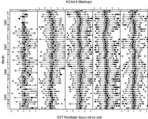
|
|||
| Figure 4b. Boxplots of Pathfinder SST residuals for NOAA-11, November 1988 to September 1994. See text for description of the plots. | ||
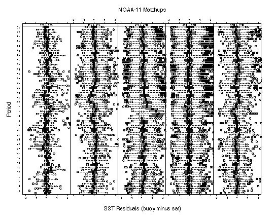
|
||
| Figure 4c. Boxplots of Pathfinder SST residuals for NOAA-9 gap period, September 1994 to March 1995. See text for description of the plots. | ||
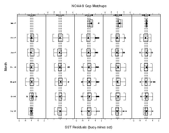
|
||
| Figure 4d. Boxplots of Pathfinder SST residuals for NOAA-14, February 1995 to December 1995. See text for description of the plots. | ||
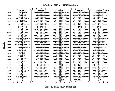
|
||
Global vs. Regional AlgorithmsThe main challenge in developing a Pathfinder global SST algorithm is to achieve relatively uniform performance throughout a wide range of atmospheric and oceanic conditions. As Barton [1995] pointed out, SST algorithms assume a first guess of the state of the atmosphere (e.g., a typical shape of water vapor and temperature profiles). A similar statement can be made about typical oceanic conditions (e.g., a certain average structure of the ocean's uppermost layer is assumed in comparisons with in situ SST measurements). When conditions deviate from the implicit first guess in atmosphere and ocean conditions, errors arise in SST retrievals. Deviations from implicit first-guess conditions are more likely in a global algorithm than in regionally-tuned algorithms, and this should be kept in mind when evaluating global SST estimates. Furthermore, in the case of statistically-derived global SST algorithms, the first-guess conditions will be the average of conditions at all the matchup locations and times used in coefficient estimation. We stress that this average will be weighted by the relative distribution of matchups, likely to change in time. The performance of an SST algorithm for a given set of atmospheric and oceanic conditions, therefore, depends not only on how close those conditions are to the average state, but also on how well represented are those conditions in the matchup set used to derived the algorithm coefficients. ReferencesAnding, D, and R. Kauth. 1970. Estimation of sea surface temperature from space. Remote Sensing of the Environment 1: 217-220. Barton, I.J., 1995. Satellite-derived sea surface temperatures: Current status. Journal of Geophysical Research 100: 87778790. Barton, I.J. and R.P. Cechet. 1989. Comparison and optimization of AVHRR sea surface temperature algorithms. Journal of Atmospheric and Oceanic Technology 6: 10831089. Cayula, J.-F. and P. Cornillon. 1996. Cloud detection from a sequence of SST images. Remote Sensing of the Environment 55: 8088. Cornillon, P., C. Gilman, C., L. Stramma, O. Brown, R. Evans and J. Brown. 1987. Processing and analysis of large volumes of satellite-derived thermal infrared data. Journal of Geophysical Research 92: 12,99313,002. Derrien, M., B. Farki, L. Harang, H. LeGléau, A. Noyalet, D. Pochic and A. Sairouni. Automatic cloud detection applied to NOAA-11/AVHRR imagery. Remote Sensing of the Environment 46: 246267. |
||
| Emery, W.J., Y. Yu, G.A.
Wick, P. Schluessel and R.W. Reynolds. 1994. Correcting infrared satellite
estimates of sea surface temperature for atmospheric water vapor contamination.
Journal of Geophysical Research 99: 52195236.
Lanzante, J.R. 1996. Resistant, robust and non-parametric techniques for the analysis of climate data: Theory and examples, including applications to historical radiosonde station data. International Journal of Climatology 16: 11971226. Luo, G., P.A. Davis, L.B. Stowe and E.P. McClain. 1995. A pixel-scale algorithm of cloud type, layer and amount for AVHRR data. Part I: Nightime. Journal of Atmospheric and Oceanic Technology 12: 10131037. McClain, E.P., W.G. Pichel and C.C. Walton. 1985. Comparative performance of AVHRR-based multichannel sea surface temperatures. Journal of Geophysical Research 90: 11,58711,601. Minnett, P.J. 1990. The regional optimisation of infrared measurements of sea surface temperature from space. Journal of Geophysical Research 95: 13,49713,510. Prabhakara, C., G. Dalu and V.G. Kunde. 1974. Estimation of sea surface temperature from remote sensing in the 11 to 13-um window region. Journal of Geophysical research 79: 5039-5044. Rousseeuw, P.J. and A.M. Leroy. 1987. Robust regression and outlier detection. John Wiley & Sons. New York. 329 p. Saunders, R.W. and K.T. Kriebel. 1988. An improved method for detecting clear sky and cloudy radiances from AVHRR data. International Journal of Remote Sensing 9: 123150. Schwalb, A. 1978. The TIROS-N/NOAA A-G satellite series. NOAA Technical Memorandum NESS 95. U.S. Government Printing Office. Washington, DC. 75 p. Walton, C.C. 1988. Nonlinear multichannel algorithm for estimating sea surface temperature with AVHRR satellite data. Journal of Applied Meteorology 27: 115124. Walton, C.C., E.P. McClain and J.F. Sapper. 1990. Recent changes in satellite based multichannel sea surface temperature algorithms. Marine Technology Society Meeting, MTS' 90, Washington D.C, September 1990. Wick, G.A., W.J. Emery and P. Schluessel. 1992. A comprehensive comparison between satellite-measured skin and multichannel sea surface temperature. Journal of Geophysical Research 97: 55695595. |
||
Appendix APathfinder V4 SST Algorithm coefficients A.1 Coefficients for NOAA-9. The second and third columns show the beginning and end dates for which each set of coefficients should be used (dates expressed as year-day of year). For each period, two rows are shown, one for coefficients used in low water vapor regimes (T4T5 0.7°C) and the other one for coefficients used in medium/high water vapor regimes (T4 - T5 > 0.7°C). The coefficients a, b, c and d correspond to the algorithm form shown in the text. AVHRR T4 - T5 Begin End a b c d
regime date date
|
||
NOA9 0.7° 85001 85031 1.220 0.965 0.127 1.191 NOA9 > 0.7° 85001 85031 1.487 0.980 0.077 1.085 NOA9 0.7° 85032 85059 1.199 0.957 0.142 1.182 NOA9 > 0.7° 85032 85059 1.513 0.979 0.077 1.080 NOA9 0.7° 85060 85090 1.244 0.941 0.161 1.203 NOA9 > 0.7° 85060 85090 1.506 0.976 0.080 1.061 NOA9 0.7° 85091 85120 1.180 0.934 0.182 1.230 NOA9 > 0.7° 85091 85120 1.499 0.978 0.079 1.078 NOA9 0.7° 85121 85151 1.160 0.936 0.176 1.251 NOA9 > 0.7° 85121 85151 1.471 0.976 0.081 1.083 NOA9 0.7° 85152 85181 1.147 0.939 0.160 1.375 NOA9 > 0.7° 85152 85181 1.432 0.973 0.084 1.016 NOA9 0.7° 85182 85212 1.301 0.922 0.154 1.278 NOA9 > 0.7° 85182 85212 1.496 0.967 0.083 0.988 NOA9 0.7° 85213 85243 1.136 0.943 0.132 1.226 NOA9 > 0.7° 85213 85243 1.453 0.963 0.086 0.958 NOA9 0.7° 85244 85273 1.316 0.927 0.140 1.061 NOA9 > 0.7° 85244 85273 1.346 0.965 0.087 0.915 NOA9 0.7° 85274 85304 1.148 0.938 0.147 0.672 NOA9 > 0.7° 85274 85304 1.248 0.971 0.087 0.911 NOA9 0.7° 85305 85334 1.316 0.919 0.166 0.307 NOA9 > 0.7° 85305 85334 1.235 0.978 0.084 0.930 NOA9 0.7° 85335 85365 1.386 0.919 0.163 0.191 NOA9 > 0.7° 85335 85365 1.282 0.975 0.084 1.011 NOA9 0.7° 86001 86031 1.361 0.931 0.152 0.083 NOA9 > 0.7° 86001 86031 1.316 0.983 0.079 1.070 NOA9 0.7° 86032 86059 1.346 0.935 0.147 0.363 NOA9 > 0.7° 86032 86059 1.370 0.981 0.079 1.071 NOA9 0.7° 86060 86090 1.368 0.936 0.141 0.959 NOA9 > 0.7° 86060 86090 1.408 0.979 0.080 1.056 |
||
AVHRR     T4 - T5     Begin         End     a     b     c     d
     regime        date           date
|
||
NOA9 0.7° 86091 86120 1.363 0.929 0.148 1.176 NOA9 > 0.7° 86091 86120 1.388 0.976 0.083 1.071 NOA9 0.7° 86121 86151 1.384 0.920 0.157 1.219 NOA9 > 0.7° 86121 86151 1.409 0.975 0.083 1.130 NOA9 0.7° 86152 86181 1.401 0.915 0.159 1.305 NOA9 > 0.7° 86152 86181 1.477 0.976 0.080 1.149 NOA9 0.7° 86182 86212 1.282 0.915 0.168 1.376 NOA9 > 0.7° 86182 86212 1.421 0.983 0.077 1.146 NOA9 0.7° 86213 86243 1.186 0.918 0.175 1.141 NOA9 > 0.7° 86213 86243 1.392 0.983 0.077 1.095 NOA9 0.7° 86244 86273 1.246 0.911 0.181 0.768 NOA9 > 0.7° 86244 86273 1.311 0.983 0.079 1.068 NOA9 0.7° 86274 86304 1.417 0.887 0.201 0.695 NOA9 > 0.7° 86274 86304 1.341 0.974 0.082 1.034 NOA9 0.7° 86305 86334 1.605 0.879 0.200 -0.203 NOA9 > 0.7° 86305 86334 1.442 0.962 0.087 0.929 NOA9 0.7° 86335 86365 1.551 0.912 0.152 0.569 NOA9 > 0.7° 86335 86365 1.585 0.952 0.089 0.865 NOA9 0.7° 87001 87031 1.505 0.920 0.147 0.605 NOA9 > 0.7° 87001 87031 1.629 0.948 0.090 0.871 NOA9 0.7° 87032 87059 1.456 0.908 0.173 0.725 NOA9 > 0.7° 87032 87059 1.647 0.950 0.089 0.890 NOA9 0.7° 87060 87090 1.415 0.901 0.193 0.558 NOA9 > 0.7° 87060 87090 1.672 0.956 0.086 0.882 NOA9 0.7° 87087 91120 1.398 0.896 0.204 0.390 NOA9 > 0.7° 87087 91120 1.611 0.963 0.084 0.922 NOA9 0.7° 87121 87151 1.379 0.899 0.199 0.297 NOA9 > 0.7° 87121 87151 1.501 0.975 0.082 0.952 NOA9 0.7° 87152 87181 1.182 0.917 0.199 0.507 NOA9 > 0.7° 87152 87181 1.514 0.979 0.079 0.974 NOA9 0.7° 87182 87212 1.248 0.911 0.194 0.326 NOA9 > 0.7° 87182 87212 1.569 0.973 0.080 0.953 NOA9 0.7° 87213 87243 1.251 0.908 0.191 0.363 NOA9 > 0.7° 87213 87243 1.476 0.972 0.081 0.855 NOA9 0.7° 87244 87273 1.399 0.894 0.199 0.059 NOA9 > 0.7° 87244 87273 1.462 0.965 0.083 0.800 NOA9 0.7° 87274 87304 1.508 0.901 0.176 0.216 NOA9 > 0.7° 87274 87304 1.419 0.963 0.085 0.760 NOA9 0.7° 87305 87334 1.585 0.874 0.211 -0.241 NOA9 > 0.7° 87305 87334 1.452 0.962 0.085 0.755 NOA9 0.7° 87335 87365 1.537 0.894 0.183 -0.047 NOA9 > 0.7° 87335 87365 1.475 0.959 0.087 0.730 |
||
AVHRR     T4 - T5     Begin     End     a     b     c     d
     regime     date     date
|
||
NOA9 0.7° 88001 88031 1.500 0.910 0.164 -0.414 NOA9 > 0.7° 88001 88031 1.488 0.958 0.087 0.764 NOA9 0.7° 88032 88060 1.509 0.907 0.161 -0.375 NOA9 > 0.7° 88032 88060 1.561 0.951 0.089 0.748 NOA9 0.7° 88061 88091 1.506 0.915 0.148 -0.246 NOA9 > 0.7° 88061 88091 1.556 0.950 0.089 0.762 NOA9 0.7° 88088 92121 1.487 0.905 0.168 -0.277 NOA9 > 0.7° 88088 92121 1.545 0.954 0.088 0.784 NOA9 0.7° 88122 88152 1.489 0.907 0.163 -0.175 NOA9 > 0.7° 88122 88152 1.504 0.965 0.083 0.842 NOA9 0.7° 88153 88182 1.468 0.898 0.179 0.156 NOA9 > 0.7° 88153 88182 1.531 0.969 0.080 0.872 NOA9 0.7° 88183 88213 1.325 0.918 0.165 0.081 NOA9 > 0.7° 88183 88213 1.569 0.968 0.080 0.851 NOA9 0.7° 88214 88244 1.489 0.905 0.172 -0.669 NOA9 > 0.7° 88214 88244 1.647 0.968 0.079 0.767 NOA9 0.7° 88245 88274 1.500 0.919 0.154 -0.998 NOA9 > 0.7° 88245 88274 1.693 0.962 0.081 0.671 NOA9 0.7° 88275 88305 1.642 0.909 0.161 -1.436 NOA9 > 0.7° 88275 88305 1.796 0.950 0.084 0.595 NOA9 0.7° 88306 88335 1.638 0.918 0.152 -1.418 NOA9 > 0.7° 88306 88335 1.840 0.943 0.085 0.560 |
||
A.2 Coefficients for NOAA-11.
The second and third columns show the beginning and end dates for which
each set of coefficients should be used (dates expressed as year-day of
year). For each period, two rows are shown, one for coefficients used in
low water vapor regimes (T4T5 0.7°C) and the other one for coefficients
used in medium/high water vapor regimes (T4 - T5 > 0.7°C). The coefficients
a, b, c and d correspond to the algorithm form shown in the text.
AVHRR     T4 - T5     Begin     End     a     b     c     d
     regime     date     date
|
||
NO11 0.7° 88306 88335 0.979 0.920 0.171 0.720 NO11 > 0.7° 88306 88335 1.146 0.964 0.081 0.941 NO11 0.7° 88336 88366 1.120 0.895 0.193 0.643 NO11 > 0.7° 88336 88366 1.226 0.960 0.081 0.950 NO11 0.7° 89001 89031 1.213 0.886 0.198 0.707 NO11 > 0.7° 89001 89031 1.261 0.958 0.081 0.962 NO11 0.7° 89032 89059 1.307 0.895 0.178 0.760 NO11 > 0.7° 89032 89059 1.374 0.952 0.082 0.952 NO11 0.7° 89060 89090 1.374 0.901 0.167 0.782 NO11 > 0.7° 89060 89090 1.455 0.948 0.081 0.954 NO11 0.7° 89091 89120 1.455 0.900 0.162 0.719 NO11 > 0.7° 89091 89120 1.541 0.944 0.081 0.954 NO11 0.7° 89121 89151 1.508 0.887 0.181 0.529 NO11 > 0.7° 89121 89151 1.58: 0.947 0.079 0.966 NO11 0.7° 89152 89181 1.592 0.876 0.186 0.386 NO11 > 0.7° 89152 89181 1.654 0.951 0.075 0.986 NO11 0.7° 89182 89212 1.771 0.855 0.175 0.614 NO11 > 0.7° 89182 89212 1.56: 0.959 0.073 0.991 NO11 0.7° 89213 89243 1.645 0.873 0.147 0.886 NO11 > 0.7° 89213 89243 1.369 0.969 0.072 0.986 NO11 0.7° 89244 89273 1.221 0.906 0.145 0.819 NO11 > 0.7° 89244 89273 1.206 0.974 0.073 0.972 NO11 0.7° 89274 89304 0.908 0.93: 0.139 0.732 NO11 > 0.7° 89274 89304 1.079 0.977 0.074 0.975 NO11 0.7° 89305 89334 0.891 0.948 0.134 0.808 NO11 > 0.7° 89305 89334 1.125 0.971 0.077 0.960 NO11 0.7° 89335 89365 0.967 0.950 0.127 0.959 NO11 > 0.7° 89335 89365 1.250 0.961 0.079 0.930 NO11 0.7° 90001 90031 1.117 0.942 0.124 1.088 NO11 > 0.7° 90001 90031 1.387 0.955 0.079 0.918 NO11 0.7° 90032 90059 1.214 0.932 0.130 1.091 NO11 > 0.7° 90032 90059 1.503 0.950 0.079 0.920 NO11 0.7° 90060 90090 1.114 0.960 0.105 1.535 NO11 > 0.7° 90060 90090 1.543 0.949 0.079 0.936 |
||
AVHRR     T4 - T5     Begin     End     a     b     c     d
     regime     date     date
|
||
NO11 0.7° 90091 90120 1.004 0.984 0.075 1.926 NO11 > 0.7° 90091 90120 1.533 0.950 0.078 0.944 NO11 0.7° 90121 90151 0.925 0.991 0.066 2.148 NO11 > 0.7° 90121 90151 1.465 0.957 0.077 0.968 NO11 0.7° 90152 90181 0.885 0.993 0.060 2.148 NO11 > 0.7° 90152 90181 1.392 0.962 0.076 0.994 NO11 0.7° 90182 90212 0.961 0.985 0.064 1.836 NO11 > 0.7° 90182 90212 1.301 0.969 0.074 1.004 NO11 0.7° 90213 90243 1.197 0.965 0.073 1.225 NO11 > 0.7° 90213 90243 1.341 0.965 0.074 1.001 NO11 0.7° 90244 90273 1.551 0.904 0.131 0.635 NO11 > 0.7° 90244 90273 1.333 0.963 0.075 0.982 NO11 0.7° 90274 90304 1.460 0.911 0.132 0.526 NO11 > 0.7° 90274 90304 1.374 0.958 0.077 0.941 NO11 0.7° 90305 90334 1.404 0.917 0.126 0.670 NO11 > 0.7° 90305 90334 1.382 0.955 0.079 0.906 NO11 0.7° 90335 90365 1.361 0.917 0.129 0.997 NO11 > 0.7° 90335 90365 1.397 0.950 0.081 0.895 NO11 0.7° 91001 91031 1.356 0.921 0.120 1.233 NO11 > 0.7° 91001 91031 1.411 0.949 0.082 0.905 NO11 0.7° 91032 91059 1.328 0.928 0.113 1.391 NO11 > 0.7° 91032 91059 1.462 0.946 0.082 0.946 NO11 0.7° 91060 91090 1.363 0.929 0.108 1.410 NO11 > 0.7° 91060 91090 1.465 0.947 0.080 0.987 NO11 0.7° 91091 91120 1.380 0.927 0.113 1.229 NO11 > 0.7° 91091 91120 1.483 0.948 0.079 0.992 NO11 0.7° 91121 91151 1.403 0.929 0.112 1.122 NO11 > 0.7° 91121 91151 1.474 0.951 0.078 1.004 NO11 0.7° 91151 91166 1.389 0.923 0.129 0.910 NO11 > 0.7° 91151 91166 1.474 0.954 0.076 1.005 NO11 0.7° 91167 91181 1.586 0.897 0.162 0.933 NO11 > 0.7° 91167 91181 1.454 0.969 0.077 0.962 NO11 0.7° 91182 91212 1.622 0.915 0.133 1.454 NO11 > 0.7° 91182 91212 1.528 0.965 0.078 0.952 NO11 0.7° 91213 91243 1.762 0.908 0.130 1.443 NO11 > 0.7° 91213 91243 1.502 0.966 0.080 0.950 NO11 0.7° 91244 91273 1.864 0.906 0.124 1.414 NO11 > 0.7° 91244 91273 1.528 0.963 0.083 0.934 NO11 0.7° 91274 91304 1.936 0.896 0.137 1.287 NO11 > 0.7° 91274 91304 1.575 0.959 0.086 0.933 NO11 0.7° 91305 91334 1.942 0.897 0.145 1.357 NO11 > 0.7° 91305 91334 1.616 0.962 0.086 0.962 |
||
AVHRR     T4 - T5     Begin     End     a     b     c     d
     regime     date     date
|
||
NO11 0.7° 91335 91365 1.947 0.902 0.148 1.327 NO11 > 0.7° 91335 91365 1.621 0.968 0.084 1.020 NO11 0.7° 92001 92031 1.928 0.919 0.134 1.516 NO11 > 0.7° 92001 92031 1.783 0.965 0.082 1.044 NO11 0.7° 92032 92060 1.950 0.929 0.122 1.658 NO11 > 0.7° 92032 92060 1.920 0.959 0.081 1.062 NO11 0.7° 92061 92091 1.992 0.934 0.113 1.690 NO11 > 0.7° 92061 92091 2.058 0.952 0.080 1.083 NO11 0.7° 92092 92121 2.043 0.935 0.108 1.639 NO11 > 0.7° 92092 92121 2.212 0.944 0.080 1.108 NO11 0.7° 92122 92152 2.103 0.934 0.105 1.604 NO11 > 0.7° 92122 92152 2.317 0.93: 0.079 1.125 NO11 0.7° 92153 92182 2.177 0.926 0.106 1.521 NO11 > 0.7° 92153 92182 2.275 0.945 0.077 1.125 NO11 0.7° 92183 92213 2.234 0.912 0.118 1.493 NO11 > 0.7° 92183 92213 2.200 0.949 0.076 1.115 NO11 0.7° 92214 92244 2.226 0.901 0.128 1.360 NO11 > 0.7° 92214 92244 2.083 0.951 0.076 1.065 NO11 0.7° 92245 92274 2.212 0.886 0.146 1.200 NO11 > 0.7° 92245 92274 2.072 0.947 0.077 0.995 NO11 0.7° 92275 92305 2.180 0.883 0.149 0.991 NO11 > 0.7° 92275 92305 2.100 0.93: 0.079 0.933 NO11 0.7° 92306 92335 2.182 0.886 0.138 0.991 NO11 > 0.7° 92306 92335 2.150 0.934 0.079 0.905 NO11 0.7° 92336 92366 2.158 0.894 0.123 1.131 NO11 > 0.7° 92336 92366 2.155 0.934 0.078 0.902 NO11 0.7° 93001 93031 2.088 0.901 0.118 1.267 NO11 > 0.7° 93001 93031 2.164 0.933 0.076 0.896 NO11 0.7° 93032 93059 2.034 0.914 0.105 1.336 NO11 > 0.7° 93032 93059 2.176 0.930 0.077 0.872 NO11 0.7° 93060 93090 2.006 0.914 0.109 1.271 NO11 > 0.7° 93060 93090 2.173 0.928 0.077 0.856 NO11 0.7° 93091 93120 1.972 0.911 0.117 1.070 NO11 > 0.7° 93091 93120 2.128 0.929 0.078 0.845 NO11 0.7° 93121 93151 1.910 0.912 0.119 0.950 NO11 > 0.7° 93121 93151 2.060 0.933 0.077 0.858 NO11 0.7° 93152 93181 1.828 0.908 0.130 0.777 NO11 > 0.7° 93152 93181 1.980 0.936 0.077 0.856 NO11 0.7° 93182 93212 1.693 0.907 0.133 0.812 NO11 > 0.7° 93182 93212 1.897 0.938 0.077 0.806 |
||
AVHRR     T4 - T5     Begin     End     a     b     c     d
     regime     date     date
|
||
NO11 0.7° 93213 93243 1.714 0.901 0.137 0.625 NO11 > 0.7° 93213 93243 1.805 0.938 0.078 0.712 NO11 0.7° 93244 93273 1.833 0.889 0.140 0.505 NO11 > 0.7° 93244 93273 1.866 0.931 0.080 0.606 NO11 0.7° 93274 93304 1.955 0.878 0.144 0.089 NO11 > 0.7° 93274 93304 1.997 0.921 0.081 0.508 NO11 0.7° 93305 93334 2.090 0.869 0.144 -0.377 NO11 > 0.7° 93305 93334 2.130 0.913 0.082 0.440 NO11 0.7° 93335 93365 2.140 0.880 0.127 -0.674 NO11 > 0.7° 93335 93365 2.178 0.912 0.083 0.399 NO11 0.7° 94001 94031 2.077 0.891 0.124 -1.179 NO11 > 0.7° 94001 94031 2.148 0.916 0.082 0.396 NO11 0.7° 94032 94059 1.910 0.912 0.119 -0.473 NO11 > 0.7° 94032 94059 2.119 0.919 0.081 0.405 NO11 0.7° 94060 94090 1.828 0.910 0.137 -0.263 NO11 > 0.7° 94060 94090 2.071 0.924 0.080 0.460 NO11 0.7° 94091 94120 1.792 0.908 0.147 -0.094 NO11 > 0.7° 94091 94120 2.030 0.928 0.078 0.528 NO11 0.7° 94121 94151 1.725 0.912 0.150 0.156 NO11 > 0.7° 94121 94151 2.004 0.932 0.077 0.604 NO11 0.7° 94152 94181 1.706 0.914 0.153 0.287 NO11 > 0.7° 94152 94181 2.100 0.929 0.076 0.626 NO11 0.7° 94182 94212 1.691 0.916 0.150 0.495 NO11 > 0.7° 94182 94212 2.154 0.926 0.075 0.627 NO11 0.7° 94213 94243 1.722 0.918 0.144 0.708 NO11 > 0.7° 94213 94243 2.245 0.921 0.075 0.597 NO11 0.7° 94244 94273 1.722 0.922 0.135 1.259 NO11 > 0.7° 94244 94273 2.261 0.921 0.075 0.581 |
||
A.3 Coefficients for NOAA-9,
gap period. The second and third columns show the beginning and end dates
for which each set of coefficients should be used (dates expressed as year-day
of year). For each period, two rows are shown, one for coefficients used
in low water vapor regimes (T4T5 0.7°C) and the other one for
coefficients used in medium/high water vapor regimes (T4 - T5 > 0.7°C).
The coefficients a, b, c and d correspond to the algorithm form shown in
the text. Note that in this case only one set of coefficients (per T45
regime) was used for the entire period (i.e., no monthly coefficients were
used).
AVHRR     T4 - T5     Begin     End     a     b     c     d
     regime     date     date
|
||
NOA9g 0.7° 94244 95120 1.439 0.902 0.188 0.913 NOA9g > 0.7° 94244 95120 1.656 0.970 0.079 1.043 |
||
A.4 Coefficients for NOAA-14.
The second and third columns show the beginning and end dates for which
each set of coefficients should be used (dates expressed as year-day of
year). For each period, two rows are shown, one for coefficients used in
low water vapor regimes (T4T5 0.7°C) and the other one for coefficients
used in medium/high water vapor regimes (T4 - T5 > 0.7°C). The coefficients
a, b, c and d correspond to the algorithm form shown in the text.
AVHRR     T4 - T5     Begin     End     a     b     c     d
     regime     date     date
|
||
NO14 0.7° 95001 95059 1.013 0.931 0.108 0.832 NO14 > 0.7° 95001 95059 1.273 0.951 0.074 0.894 NO14 0.7° 95060 95090 1.050 0.921 0.121 1.220 NO14 > 0.7° 95060 95090 1.242 0.955 0.072 0.909 NO14 0.7° 95091 95120 1.049 0.907 0.141 1.218 NO14 > 0.7° 95091 95120 1.235 0.957 0.072 0.911 NO14 0.7° 95121 95151 1.045 0.904 0.152 1.114 NO14 > 0.7° 95121 95151 1.258 0.956 0.072 0.905 NO14 0.7° 95152 95181 1.084 0.899 0.152 1.094 NO14 > 0.7° 95152 95181 1.250 0.959 0.071 0.921 NO14 0.7° 95182 95212 1.062 0.901 0.149 1.068 NO14 > 0.7° 95182 95212 1.286 0.958 0.070 0.897 NO14 0.7° 95213 95243 0.978 0.908 0.142 1.161 NO14 > 0.7° 95213 95243 1.299 0.956 0.070 0.894 NO14 0.7° 95244 95273 0.949 0.913 0.134 1.195 NO14 > 0.7° 95244 95273 1.325 0.951 0.071 0.894 NO14 0.7° 95274 95304 0.989 0.912 0.129 1.355 NO14 > 0.7° 95274 95304 1.335 0.948 0.072 0.906 NO14 0.7° 95305 95334 1.077 0.912 0.117 0.896 NO14 > 0.7° 95305 95334 1.350 0.949 0.071 0.892 NO14 0.7° 95335 95365 1.163 0.905 0.117 0.971 NO14 > 0.7° 95335 95365 1.372 0.946 0.073 0.873 NO14 0.7° 96001 96059 1.013 0.931 0.108 0.832 NO14 > 0.7° 96001 96059 1.273 0.951 0.074 0.894 NO14 0.7° 96060 96090 1.050 0.921 0.121 1.220 NO14 > 0.7° 96060 96090 1.242 0.955 0.072 0.909 NO14 0.7° 96091 96120 1.049 0.907 0.141 1.218 NO14 > 0.7° 96091 96120 1.235 0.957 0.072 0.911 NO14 0.7° 96121 96151 1.045 0.904 0.152 1.114 NO14 > 0.7° 96121 96151 1.258 0.956 0.072 0.905 NO14 0.7° 96152 96181 1.084 0.899 0.152 1.094 NO14 > 0.7° 96152 96181 1.250 0.959 0.071 0.921 NO14 0.7° 96182 96212 1.062 0.901 0.149 1.068 NO14 > 0.7° 96182 96212 1.286 0.958 0.070 0.897 |
||
AVHRR     T4 - T5     Begin     End     a     b     c     d
     regime     date     date
|
||
NO14 0.7° 96213 96243 0.978 0.908 0.142 1.161 NO14 > 0.7° 96213 96243 1.299 0.956 0.070 0.894 NO14 0.7° 96244 96273 0.949 0.913 0.134 1.195 NO14 > 0.7° 96244 96273 1.325 0.951 0.071 0.894 NO14 0.7° 96274 96304 0.989 0.912 0.129 1.355 NO14 > 0.7° 96274 96304 1.335 0.948 0.072 0.906 NO14 0.7° 96305 96334 1.077 0.912 0.117 0.896 NO14 > 0.7° 96305 96334 1.350 0.949 0.071 0.892 NO14 0.7° 96335 96365 1.163 0.905 0.117 0.971 NO14 > 0.7° 96335 96365 1.372 0.946 0.073 0.873 |
||
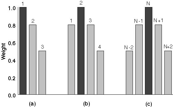
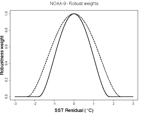
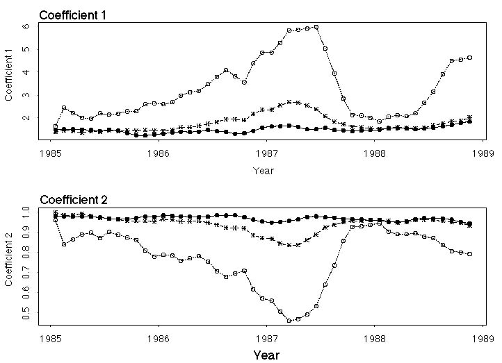